| Issue |
A&A
Volume 651, July 2021
|
|
|---|---|---|
| Article Number | A110 | |
| Number of page(s) | 7 | |
| Section | Planets and planetary systems | |
| DOI | https://doi.org/10.1051/0004-6361/202038844 | |
| Published online | 27 July 2021 | |
A lighter core for Phobos?
1
State Key Laboratory of Information Engineering in Surveying, Mapping and Remote sensing,
Wuhan,
PR China
e-mail: This email address is being protected from spambots. You need JavaScript enabled to view it.
2
Institute of Space Technology and Space Applications, Universität der Bundeswehr München,
Neubiberg,
Germany
3
Rheinisches Institut für Umweltforschung, Abteilung Planetenforschung, an der Universität zu Köln,
Köln,
Germany
4
Geodesy Observatory of Tahiti, University of French Polynesia,
BP 6570,
98702
Faaa,
Tahiti, French Polynesia,
France
Received:
4
July
2020
Accepted:
6
May
2021
Abstract
Context. The origin of the Martian moons Phobos and Deimos is still poorly understood, and is the focus of intense debate.
Aims. We demonstrate that a stratified internal structure of Phobos is compatible with the observed gravity coefficients.
Methods. We fit previously derived C20 and C22 Phobos gravity coefficients derived from the combined MEX Doppler-tracking data from the close flybys in +2010 and 2013 with respect to the corresponding coefficients of a core–mantle stratification model of Phobos, with two opposite cases: a core denser than the mantle, and a core lighter than the mantle.
Results. Only the case with a core lighter than the mantle fits at the 3σ level the previously reported observed second degree and order coefficient C20, but a homogeneous Phobos cannot be strictly ruled out at the 3σ level.
Conclusions. This possible loosening of the core density might be the result of a displacement of material toward the surface, may be caused by centrifugal forces acting on a loosely packed rubble-pile structure, and/or by a hot-then-cold in-orbit accretion process. These two hypotheses are by no means exhaustive.
Key words: gravitation / planets and satellites: formation
© ESO 2021
1 Introduction
Two possible origins for the Phobos and Deimos moons of Mars are discussed in the literature: capture or in situ formation by accretion of debris that was transported into orbit after a strong impact by an asteroid on Mars (Rosenblatt et al. 2020). Evidence also argues for several cycles of tidal disruption-reaccretion processes (Hesselbrock & Minton 2017), with the current Phobos as young as a few hundred million years (Ćuk et al. 2020). Pajola et al. (2013) indicated that the reflectance spectrum of Phobos is consistent with a D-type asteroid from the main asteroid belt, which favors the scenario that Phobos is a captured D-type asteroid. The spectrum is also compatible with the carbonaceous material of the meteorite that fell on Tagish Lake in 2000, whose parent body seems to be the D-type asteroid 773 Irmintraud (Hiroi et al. 2001). This meteorite has a bulk density of 1670 kg m−3 (Zolensky et al. 2002), a microporosity range between 4.5% and 15.4%, and a macroporosity up to 40%, with the presence of hydrated silicates (Beech & Coulson 2010). These numbers imply a density of 2700 kg m−3 for the basic material of this meteorite. Ivanov & Zolensky (2003) claimed that the meteoritic material from the Kaidun meteorite likely originated from Phobos. The porosity range of chondritic material from meteorite landfalls ranges from 0% to 53% with peaks at 0% and 4% (Corrigan et al. 1997). The capture scenario depends on the spectral analysis of the surface material on Phobos and the breaking of kinetic energy, such as the orbital tidal dissipation (Kaula 1964) or drag effect (Sasaki 1990). However, the capture theories do not work well for several reasons, and mostly fail to explain the braking of the captured asteroid into the Mars orbit. Giuranna et al. (2011) pointed out, however, that the visible and near-infrared spectra of Phobos lack deep absorption features, making any compositional interpretation a difficult task. The spectra most closely match silicate rather than chondritic materials.
If Phobos did form by accretion from debris transported into orbit after a giant impact on Mars (Craddock 2011), the bulk material of Phobos and Deimos cannot be made of primitive chondrites but rather highly brecciated material formed by shock metamorphism. The reaccretion would have occurred in such a way that the resulting bulk density corresponds to the one observed for Phobos (Yang et al. 2019, 1848 kg m−3), which is consistent with very porous chondrites. The only known in-orbit reaccretion process are those that led to the formation of the Earth’s moon, which has a bulk density of 3340 kg m−3, but on a widely different scale and density compaction by pressure at depth, and also probably those that led to the formation of asteroids Bennu and Ryugu (see thereafter). The consensus favors an in-situ formation scenario. (Craddock 2011; Richardson et al. 2002; Rosenblatt et al. 2016, 2020; Canup & Salmon 2018).
The first reliable estimate of the density of Phobos was derived by Andert et al. (2010) as 1876 ± 20 kg m−3 from a massdetermination during the Mars Express flyby at Phobos in 2008 and a volume determination from the High Resolution Stereo Camera data (HRSC, Willner et al. 2010). The most recent estimate for the density of Phobos is 1848 ± 11 kg m−3, which was derived by combining the GM estimate of 7.0765 ± 0.0075 × 10⁵ m3 s−2 obtained from modeling the Doppler shifts recorded during two flybys of the Mars Express spacecraft (Andert et al. 2010; Pätzold et al. 2014; Yang et al. 2019) and the estimate of 5742 ± 35 km3 from Willner et al. (2014). In order to explain the observed low density of Phobos, a mixture of water ice, chondritic material and/or porosity must be considered. This was already noted by Fanale & Salvail (1989), Andert et al. (2010), Rosenblatt (2011) and Pätzold et al. (2016). Lewis (2012) claimed that Phobos appears to be made of carbonaceous chondrites.
The bulk grain density for carbonaceous chondrites is about 2400 kg m−3 on average, with a microporosity as high as 35% (Consolmagno et al. 2008). The observed bulk density of Phobos is fully compatible with these microporosity values, but higher than the density of other carbonaceous asteroids visited by spacecraft. The observed bulk density for the large carbonaceous asteroid (253) Mathilde is 1300 ± 200 kg m−3. The large uncertainty in this bulk density estimates is understandable as only part of this body was photographed during the NEAR spacecraft flyby (Yeomans et al. 1997). The bulk densities of 101 955 Bennu (OSIRIS-REX mission) and 163 172 Ryugu (Hayabusa-2 mission), which are smaller carbonaceous asteroids, are 1190 ± 13 kg m−3 (Lauretta et al. 2019), and 1190 ± 20 kg m−3 (Watanabe et al. 2019), respectively. This points to either low-density materials or high porosity or both. In addition, the porosity of 433 Eros is thought to be about 20% (Wilkison et al. 2002). This high porosity is required for small bodies such as Eros to avoid catastrophic disruption by strong impacts (Richardson et al. 2002).
Several papers on the internal structure of Phobos have been published. Simulated C20 values were calculated by Pätzold et al. (2014) and Le Maistre et al. (2019). Le Maistre et al. (2019) compared several geodesic observables for four scenarios, for which the geodesic observables were obtained under the assumption that Phobos has a constant density. These four scenarios were obtained by changing the proportions of (macro-) porosity and ice. Their results favor a homogeneous porous body and tend to exclude a heavily fractured body. Nevertheless, their conclusion is to be taken with caution because the libration amplitude and the second-degree coefficients are highly correlated, and are certainly affected by the large uncertainties.
Unlike Le Maistre et al. (2019), we constrained our model of the internal structure of Phobos by comparing the computed C20 gravity coefficients with respect to the most recent accurately modeled gravity coefficients from Yang et al. (2019) and focused on a two-layer model to study the possible interior structure of Phobos. It must be stressed that comparing models to the (still-to-be-observed) inertia tensor is not equivalent to comparing models to the (observed) second-degree harmonic coefficients. There are six independent components in the inertia tensor, and only five independent coefficients for the degree two of the harmonic expansion of the gravity field. These five coefficients can be computed from the inertia tensor, but the reverse is not possible. To compute the full inertia tensor requires observations of the rotational dynamics of the body, in addition to the observed second degree gravity coefficients derived from the Doppler tracking data.
In this paper, we consider an embedded two-layer structure (a core and a mantle layer) of the Phobos interior, as a generalization of the work of Matsumoto & Ikeda (2016), who approximated Phobos using an ellipsoid model but did not consider real measurements. By varying the depth of the interface between the core and the mantle, the densities of the core and the mantle within physically reasonable values under the constraint of conservation of the total mass, sets of the second degree and order harmonic spherical gravity coefficients were computed. These sets were compared to the observed values of these gravity coefficients derived by Yang et al. (2019) from the combined MEX Doppler tracking data from the close flybys in 2010 and 2013.
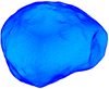 |
Fig. 1 Polyhedron model of Phobos from Willner et al. (2014) used in this study, with a mean density of 1848 kg m−3 (The density of Phobos is obtained from the GM estimate of Yang et al. 2019 and from the volume estimate of Willner et al. 2014). |
2 Observations and modeling methods
2.1 Previous shape models of Phobos
The first Phobos shape model was obtained from the data of the Mariner-9 and the Viking missions (see Table 1). In recent years, the Mars Express instruments and imagers have accumulated a large amount of high-precision data from the flyby of Phobos. The latest Phobos shape models are based on all of these data sets (Willner et al. 2010, 2014).
The shape model of Phobos from Willner et al. (2014) is widely considered as the most accurate. New models are available on several databases, but they are not yet peer-reviewed, so we used the Willner et al. (2014) model in this work (Fig. 1).
The Phobos shape model from Willner et al. (2014) is expressed as a set of harmonic coefficients corresponding to a 4 × 4 degree grid resolution on the Phobos surface. As this type of representation is not suitable for computations of the gravity from shape, we converted it into a mesh of triangles with 32 040 facets and 16 022 vertices corresponding to the spherical harmonic resolution.
2.2 Computation of the gravity harmonic coefficients for the two-layer model
To compute the gravity potential U over a sphere that completely surrounds a body(in our case, 14 km), we applied the method proposed by Werner & Scheeres (1997) that assumes a constant density in addition to a polyhedron representation of a body. We recomputed the coordinates of the vertices given by Willner et al. (2014) in the body-fixed coordinate frame used by Yang et al. (2019). The gravity potential U is defined by the usual formula,
![Mathematical equation: \begin{equation*}U\,{=}\,\frac{{GM}}{r}{\sum\limits_{l\,{=}\,0}^{\infty} {\sum\limits_{m\,{=}\,0}^l {\left({\frac{R}{r}} \right)}} ^n}{\bar P_{\textrm{lm}}}\left({\cos \varphi} \right)\left[{\bar C_{\textrm{lm}}} \cdot \cos m\lambda + {\bar S_{\textrm{lm}} \cdot \sin m\lambda} \right]\end{equation*}](/articles/aa/full_html/2021/07/aa38844-20/aa38844-20-eq1.png) (1)
(1)
where the origin of the spherical coordinate system is located in the center of mass of the body, G is the gravitational constant. M is the mass of Phobos, r is the radius distance to a test particle, and R is the radius of an embracing sphere, typically the largest axis of the body.  are the normalized Legendre polynomials, and
  and
and  are the normalized gravity field spherical harmonic coefficients.
The spherical harmonic coefficients  ,
,  were obtained by a least-squares fit from a mesh covering the sphere with several nodes tailored to the maximum degree and order of the expansion. A direct computation of the inertia tensor then of the second degree and order coefficients is of course possible (Tonon 2004), but we chose this indirect way as we are also using this gravity field model for orbit determination.
History of shape models of Phobos.
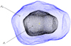 |
Fig. 2 Our Phobos two-layer model. The black part is the core with the same shape as the surface. The core is plotted in gray with a density ρc, and the mantle is plotted in blue with a density ρm. |
2.3 Method for obtaining the gravitational field of the two-layers model of Phobos
We applied the Occam razor approach (Blumer et al. 1987) by keeping the number of free parameters of our model to a minimum. We assumed two homogeneous layers (a core and a mantle) with different densities separated by an interface homothetic to the surface at a varying depth, in such a way that the mass of Phobos is maintained constant. A sketch of our two-layer model is shown in Fig. 2.
This two-layer model can be questioned ad infinitum, and especially the choice of an interface homothetic to the surface(see discussion thereafter) as well as the choice of a constant density for each layer. There is no observational evidence of an interface at depth. The only proven interface is the one between the regolith (observed surface) and the solid surface underneath. Estimates of its depth range from one meter to several dozen meters. The Bouguer map of Eros computed by Garmier et al. (2002) clearly shows a compaction of the chondritic material of Eros at the location of the main impact craters. It is therefore highly probable that some compaction also took place at the location of the Stickney crater on Phobos (Le Maistre et al. 2019). Therefore we emphasize again that our results follow the Occam razor parameterization. We discuss two main cases below: (a) a mantle denser than the core and (b) a core denser than the mantle.
For all the cases, the total mass, the total volume, and therefore the bulk density of Phobos are constants,

where MPh, Mc, Mm are respectively the masses of Phobos, the core and the mantle. VPh, Vc, Vm are respectively the volumes of Phobos, the core and the mantle. Therefore,

where ρbulk, ρc, and ρm are the bulk densities of Phobos, the core and the mantle, respectively. The scaling factor λ is defined as:
 (6)
(6)
When λ = 0, Vm = VPh, and when λ = 1, Vc = VPh.
The interface depth d represents the mean thickness of the mantle,
 (7)
(7)
Here (xn, yn, zn) is the coordinate of a given point of the Phobos shape model and n is the number of the points. The density of the mantle ρm depends on the density of the core ρc by
 (8)
(8)
We limited the range of possible core density values to the two extreme cases found in the literature. A minimum density of 500 kg m−3, as found for cometarity nuclei such as 67P/Churyumov-Gerasimenko (533 ± 6 kg m−3, Pätzold et al. 2016), and a maximum density of 5000 kg m−3 as found for asteroid (216) Kleopatra from the motion of its moons (4900 ± 500 kg m−3, Shepard et al. 2018).
The potential U for different layering cases of Phobos were calculated by the following relation:
 (9)
(9)
Here  ,
,  is the potential from the scaled core with constant densities ρc or ρm, and UPh is the potential from the polyhedron model of Phobos with a constant density ρm.
Measured values of the Phobos  and
and  normalized gravity coefficients from the MEX two-way Doppler data acquired during the 2010 and 2013 flybys and the corresponding gravity coefficients for a homogeneous Phobos.
3 Computation results and analysis
3.1 Observed values for C20 and C22
Matsumoto & Ikeda (2016) claimed that the required accuracy for the second-degree and order gravity coefficients needs to reach a few percent if we wish to constrain the inhomogeneous interior structure of Phobos. Le Maistre et al. (2019) considered that a determination of C20 and C22 at the 5% level or better would corroborate the conclusions drawn from the libration estimates. Pätzold et al. (2014) published estimates of C20 and C22 from the 2010 flyby, but with larger error bars than those in the work of Yang et al. (2019). Table 2 clearly indicates that the combination of the tracking data from the 2010 and 2013 flybys was the key factor to improve these error bars. Therefore we considered the C20 and C22 estimates from Yang et al. (2019).
3.2 Results for the Phobos interior structure
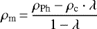
Figure 3 shows the relation between the core and mantle densities for selected values of  according toEq. (8). We chose six values for the scaling size of the core, 0.1, 0.2, 0.4, 0.6, 0.8, 0.9. All lines cross at point A which is the bulk density of a homogeneous Phobos.
For core densities lower than the bulk density (left of point A shown in Fig. 3), the mantle is denser than the core, and vice versa, for core densities higher than the bulk density (right of point A), the mantle is less dense than the core. Figures 4a and 4b show the dependence of the mantle density on the size of the core for selected core densities.
In Fig. 4, only physical values (from 500 kg m−3 to 5000 kg m−3) for the densities of the mantle and the core are listed. For a given scaling factor of the core λ and the density of the core ρc, 46 layering cases are considered in this paper. We removed the cases exceeding the allowable density range.
Plots in Figs. 5 and 6 show that at the 3σ level, the modeled and observed C20 agree well when the mantle is denser than the core (see also Tables 3 and 4).
To verify the effect of the core shape on the gravity field of the two-layer Phobos model, we used a triaxial ellipsoid core shape (homotheticto the best-fit triaxial ellipsoid of Phobos (Willner et al. 2014), and recalculated the second-degree coefficients in a setting identical to the one used for Figs. 5 and 6. The gravity potential of a homogeneous ellipsoid canbe computed using Ivory’s formula (Garmier et al. 2002). Compared to the minimum absolute value of  from Yang et al. (2019), when the mantle is denser than the core, the cases listed in Table 3 (homothetic surface shapes) and Table 5 (homothetic ellipsoids) coincide. A test simulation for a core with a scaling factor of 0.6 and a density of 1400 kg m−3 produced a very small deviation
  of 0.097%, therefore, the deviation
  is not sensitive to the core shape, if the interface core-mantle is deeply buried. Only one test simulation is compatible with the data when the core is denser than the mantle. In this case, the core had a scaling factor of 0.1 and a density of 2200 kg m−3, and the corresponding deviation
  was 0.002%.These results are summarized in Tables 5 and 6.
The disrupted and reaccreted body (DAR-F1) model (a rubble-pile internal structure), with a denser outer layer considered by Le Maistre et al. (2019), is close to our two-layer model for a core with a scaling factor of 0.9 (the interface depth is about 1 km).
All small bodies (radius smaller than 20 km) with known second order and degree gravity models (Miller et al. 2000; Zuber et al. 2000; Garmier et al. 2002; Hu & Jekeli 2015; Pätzold et al. 2016; Lhotka et al. 2016; Sebera et al. 2016) have a homogeneous internal structure, with the recent exception of the very small (diameter 490 m) asteroid Bennu (Scheeres et al. 2020). No results have been published so far for asteroid Ryugu. Larger asteroids or dwarf planets such as Vesta and Ceres have a differentiated structure with a core density higher than the mantle (Bland 2013; Russell et al. 2016). If a lighter core is confirmed by future observations, Phobos will be the second small body of the Solar System presenting a heterogeneous density in its interior.
A first explanation accounting for a core lighter than a mantle in Phobos could be related to the fast rotation (7.6554 h) of Phobos (Jacobson 2010) with respect to its size (mean diameter of 22 540 m (Willner et al. 2010)) and its internal cohesion. In this sense, the structure of Phobos might be similar to that of the small Bennu asteroid with a diameter of 490.06 ± 0.16 m and a rotation period of 4.296057 ± 0.000002 h (Lauretta et al. 2019). Bennu has a rubble-pile structure that seems to be caused by the aftermath disruption of its parent body or/and Yorp-induced spin (Scheeres et al. 2020). The angular momentum of Bennu was not high enough to split the body into pieces, but it was high enough for the centrifugal forces to have driven material toward the surface (Scheeres et al. 2020). The case of asteroid Ryugu seems to be similar (Michel et al. 2020; Kikuchi et al. 2021). At the equator of a nearly spherical body, centrifugal acceleration is proportional to the mean diameter of the body divided by the square of the rotation period; thus, the centrifugal acceleration of Ryugu with a rotation period 7.63262 ± 0.00002 h and a mean diameter of 870 m (Watanabe et al. 2019; Müller et al. 2011)is halved along the equator as compared to Bennu. The centrifugal acceleration on the equator of Phobos is almost 14 times higher than that on the equator of Bennu. Bennu and Ryugu exhibit circum-equatorial bulges, probably caused by centrifugal forces (Cheng et al. 2020). No such equatorial bulge is apparent on Phobos, however.
Another plausible and possibly complementary explanation for a mantle denser than the core could be a hot-then-cold accretion scenario, according to which the core of Phobos accreted in a few hours or days after an impact of a giant asteroid on Mars, with a material depleted in volatiles by the kinetic heat of the impact. After the first hot stage, a second longer accretion period involved a cooler cloud of material with significant volatile content. Rivkin et al. (2002) rejected any subsurface ice reservoir although the likely presence of outgassed water on the surface of Phobos was pointed out by Fanale & Salvail (1989) and by Kirsch et al. (1993) from observations taken by the Phobos-2 spacecraft. Radar observationsindicate that Phobos is covered by a layer of reaccreted regolith with a material density of about 1600 kg m−3 and a porosity of 40% (Busch et al. 2007). The depth of that layer is poorly constrained (Miyamoto et al. 2018, >10 m), however. Rosenblatt et al. (2016) suggested that Phobos and Deimos accreted from the outer portion of a debris disk formed after a giantasteroid impact on Mars, and that therefore both are composed of a mixture of material from Mars and the impactor (Miller et al. 2000). We can even speculate further, by suggesting that the Phobos material has essentially the same grain density for both layers, but with the interstitial space between the grains in the mantle being populated by some form of ice, therefore inducing a higher density in the mantle. When we assume a bulk density of 1600 kg m−3 and a porosity of 40% for the core, this leads to a density of 2677 kg m−3 for the core material (by applying Eq. (8) from Pätzold et al. 2014). If we assume that the mantle has the same type of structure, but with water ice filling the pores entirely, at a density of 930 kg m−3, the average density of the mantle would be around 2047 kg m−3 (by applying Eq. (8) from Pätzold et al. 2014). This results in a mantle depth of about 2000 m for a body of 10 km radius (like Phobos). The regolith layer, gradually formed by small-impact erosion and reaccretion later on acts as a thermal insulator and a seal, preventing the outgassing of the ices in the mantle. It is difficult to say more because the accretion processes, from pebbles to submeter and even larger bodies are not well understood in detail. The formation of Deimos could have followed the same scenario. The Phobos and Deimos case, with respect to planetesimals orbiting the Sun, are difficult because of the reaccretion, if any, occurred around a planetary body and not around a central star. Another disruption-reaccretion scenario is mentioned by Britt et al. (2002) and Bagheri et al. (2021). The largest pieces would have been reaccreted first, creating a large void inside the body, but without a void in the surface layer, which would have been filled by the smaller pieces in the second stage of the re-accretion process. After the reaccretion phases, Phobos and Deimos may have been separated by the altitude drift caused by the Martian tides, Phobos toward the surface of Mars, with Deimos pushed into increasingly higher orbits. We refer to Dash & Miguel (2020), Elkins-Tanton & Weiss (2017), and Ormel (2017) for reviews of our current understanding of accretion processes in solar systems, and to Rosenblatt et al. (2016) and Ćuk et al. (2020) for possible scenarios about the reaccretion of Phobos and Deimos. Even a sample from the Phobos surface, as is planned to be obtained with the MMX mission, (Kuramoto et al. 2018) will not be able to settle the case, because the regolith layer is probably deeper than what can be ascertained by any drill system. The only way to fully address the internal structure of Phobos probably is a deep-probing by radar, such as the CONSERT experiment that was conducted for the comet 67P/Churyumov-Gerasimenko (Kofman et al. 2015).
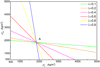 |
Fig. 3 Range of densities for the Phobos two-layer model. The x-axis is the assumed density of the core, the y-axis is the resulting density of the mantle according to Eq. (8). |
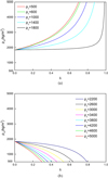 |
Fig. 4 Mantle (a) and core (b) densities as a function of the core scaling factor of Phobos’ two-layer models. (ρc is the density of the core, λ is the scalingfactor of the core, and ρm is the density of the mantle, units: kg m−3). |
 |
Fig. 5 Modeled normalized spherical harmonic coefficients C20 (black dots) and C22 (green dots) vs. the measured values by Yang et al. (2019) for the scenario where the mantle is denser than the core (the core shape is homothetic to the Phobos surface).The 1σ and 3σ error bars for the measured coefficients are the shaded and crossed bands. The different cases are shown along the y-axis: ρ_ c represents the density of the core, and |

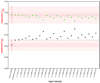 |
Fig. 6 Modeled normalized spherical harmonic coefficients C20 (black dots) and C22 (green dots) vs. the measured values from Yang et al. (2019), as in Fig. 5, but for the scenarios where the core is denser than the mantle (the core shape is homothetic to the Phobos surface). Triangles represent the layering cases that agree well with the C20 from Yang et al. (2019). The 1σ and 3σ error bars for the measured coefficients are shaded and crossed bands. Most of the modeled C20 values are outside the 3σ band around the measured value, excluding these scenarios. The case marked by a triangle is shown in Table 4. |
Three possible layering assumptions of the Phobos internal structure where the mantle is denser than the core (the core shape is homothetic to the Phobos surface).
Four possible layering assumptions of the Phobos internal structure when the mantle is denser than the core (the core shape is homothetic to the best-fit triaxial ellipsoid of Phobos; Willner et al. 2014).
Only possible layering assumption of the Phobos internal structure when the core is denser than the mantle (the core shape is homothetic to the best-fit triaxial ellipsoid of Phobos; Willner et al. 2014).
4 Conclusions
The recent estimate of Phobos C20 by Yang et al. (2019) supports an inhomogeneous distribution of matter inside Phobos in which the density decreases with depth, at a 3σ level (confidence interval of 99.7%, Yang et al. 2019). The case of a homogeneous Phobos is at the boundary of this confidence interval. In other words, a core denser than the mantle is not compatible with the current estimate of C20 by Yang et al. (2019) at the 3σ level. This might be explained by a migration of material toward the surface, either caused by centrifugal forces on a loosely packed rubble-pile small body, and/or by a hot-then-cold in-orbit accretion process with ice-rich material accreted in a second stage after an early dry-stage accretion step. This ice-rich mantle material is thereafter thermally insulated by the regolith. These two formation scenarios of Phobos are not exhaustive. We hope that the forthcoming missions might confirm our analysis.
Acknowledgements
We are grateful to NASA and ESA for providing models to make this research possible. J.Y. is supported by the pre-research Project on Civil Aerospace Technologies (No. D020103), the National Natural Science Foundation of China (42030110). M.Y. is supported by the National Natural Science Foundation of China (41804025). J.P.B. is funded by a DAR grant in planetology from the French Space Agency (CNES). T.A., M.P. and M. H. are funded by grants from the Bundesministerium für Wirtschaft and Energie, Berlin, via the German Space Agency DLR, Bonn.
References
- Andert, T., Rosenblatt, P., Pätzold, M., et al. 2010, Geophys. Res. Lett., 37, L09202 [NASA ADS] [CrossRef] [Google Scholar]
- Bagheri, A., Khan, A., Efroimsky, M., Kruglyakov, M., & Giardini, D. 2021, Nat. Astron., 5, 539 [CrossRef] [Google Scholar]
- Beech, M., & Coulson, I. M. 2010, MNRAS, 404, 1457 [Google Scholar]
- Bland, M. T. 2013, Icarus, 226, 510 [CrossRef] [Google Scholar]
- Blumer, A., Ehrenfeucht, A., Haussler, D., & Warmuth, M. K. 1987, Inform. Process. Lett., 24, 377 [CrossRef] [MathSciNet] [Google Scholar]
- Britt, D. T., Yeomans, D., Housen, K., & Consolmagno, G. 2002, Asteroids III, eds. W. F. Bottke Jr., A. Cellino, P. Paolicchi, & R. P. Binzel (Tucson: University of Arizona Press), 485 [CrossRef] [Google Scholar]
- Busch, M. W., Ostro, S. J., Benner, L. A. M., et al. 2007, Icarus, 186, 581 [CrossRef] [Google Scholar]
- Canup, R. M., & Salmon, J. 2018, Sci. Adv., 4, eaar6887 [CrossRef] [Google Scholar]
- Cheng, B., Yu, Y., Asphaug, E., et al. 2020, Nat. Astron., 5, 134 [CrossRef] [Google Scholar]
- Consolmagno, G. J., Britt, D. T., & Macke, R. J. 2008, Meteor. Planet. Sci., 43, 5038 [Google Scholar]
- Corrigan, C. M., Zolensky, M. E., Dahl, J., et al. 1997, Meteor. Planet. Sci., 32, 509 [NASA ADS] [CrossRef] [Google Scholar]
- Craddock, R. A. 2011, Icarus, 211, 1150 [CrossRef] [Google Scholar]
- Ćuk, M., Minton, D. A., Pouplin, J. L., & Wishard, C. 2020, ApJ, 896, L28 [CrossRef] [Google Scholar]
- Dash, S., & Miguel, Y. 2020, MNRAS, 499, 3510 [CrossRef] [Google Scholar]
- Duxbury, T. C. 1989, Icarus, 78, 169 [NASA ADS] [CrossRef] [Google Scholar]
- Duxbury, T. C. 1991, Planet. Space Sci., 39, 355 [NASA ADS] [CrossRef] [Google Scholar]
- Duxbury, T. C., & Veverka, J. 1977, J. Geophys. Res., 82, 4203 [CrossRef] [Google Scholar]
- Elkins-Tanton, L. T., & Weiss, B. P. 2017, Planetesimals: Early Differentiation and Consequences for Planets, Vol. 16 (Cambridge University Press) [CrossRef] [Google Scholar]
- Fanale, F. P., & Salvail, J. R. 1989, Geophys. Res. Lett., 16, 287 [NASA ADS] [CrossRef] [Google Scholar]
- Garmier, R., Barriot, J. P., Konopliv, A. S., & Yeomans, D. K. 2002, Geophys. Res. Lett., 29, 72 [CrossRef] [Google Scholar]
- Gaskell, R. 2011, Gaskell Phobos Shape Model V1.0., https://sbn.psi.edu/pds/resource/phobosshape.html [Google Scholar]
- Giuranna, M., Roush, T. L., Duxbury, T. C., et al. 2011, Planet. Space Sci., 59, 1308 [CrossRef] [Google Scholar]
- Hesselbrock, A. J., & Minton, D. A. 2017, Nat. Geosci., 10, 266 [CrossRef] [Google Scholar]
- Hiroi, T., Zolensky, M. E., & Pieters, C. M. 2001, Science, 293, 2234 [NASA ADS] [CrossRef] [PubMed] [Google Scholar]
- Hu, X., & Jekeli, C. 2015, J. Geodesy, 89, 159 [CrossRef] [Google Scholar]
- Ivanov, A., & Zolensky, M. 2003, 34th Annual Lunar Planet. Sci. Conf., March 17–21 (League City, Texas), 1236 [Google Scholar]
- Jacobson, R. A. 2010, ApJ, 139, 668 [NASA ADS] [CrossRef] [Google Scholar]
- Kaula, W. M. 1964, Rev. Geophys., 2, 661 [Google Scholar]
- Kikuchi, S., Ogawa, N., Mori, O., et al. 2021, Icarus, 358, 114220 [CrossRef] [Google Scholar]
- Kirsch, E., Mckennalawlor, S., Afonin, V. V., et al. 1993, Planet. Space Sci., 41, 435 [CrossRef] [Google Scholar]
- Kofman, W., Herique, A., Barbin, Y., et al. 2015, Science, 349, 6247 [CrossRef] [Google Scholar]
- Kuramoto, K., Kawakatsu, Y., Fujimoto, M., et al. 2018, 49th Lunar Planet. Sci. Conf., 19–23 March (The Woodlands, Texas LPI Contribution no. 2083), 2143 [Google Scholar]
- Lauretta, D. S., Dellagiustina, D. N., Bennett, C. A., et al. 2019, Nature, 568, 55 [Google Scholar]
- Le Maistre, S., Rivoldini, A., & Rosenblatt, P. 2019, Icarus, 321, 272 [NASA ADS] [CrossRef] [Google Scholar]
- Lewis, J. 2012, Physics and Chemistry of the Solar System (Academic Press) [Google Scholar]
- Lhotka, C., Reimond, S., Souchay, J., & Baur, O. 2016, MNRAS, 455, 3588 [CrossRef] [Google Scholar]
- Matsumoto, K., & Ikeda, H. 2016, 47th Lunar Planet. Sci. Conf., March 21–25 (The Woodlands, Texas. LPI Contribution No. 1903), 1846 [Google Scholar]
- Michel, P., Ballouz, R.-L., Barnouin, O., et al. 2020, Nat. Commun., 11, 1 [CrossRef] [Google Scholar]
- Miller, J. K., Antreasian, P. G., Bordi, J. J., Chesley, S., & Yeomans, D. K. 2000, in AAS/AIAA Astrodynamics Specialist Conference [Google Scholar]
- Miyamoto, H., Niihara, T., Wada, K., et al. 2018, 49th Lunar Planet. Sci. Conf., 19–23 March (The Woodlands, Texas LPI Contribution No. 2083), 1882 [Google Scholar]
- Müller, T., Ďurech, J., Hasegawa, S., et al. 2011, A&A, 525, A145 [NASA ADS] [CrossRef] [EDP Sciences] [Google Scholar]
- Ormel, C. W. 2017, Astrophys. Space Sci. Lib., 445, 197 [Google Scholar]
- Pajola, M., Lazzarin, M., Ore, C. M. D., et al. 2013, ApJ, 777, 127 [NASA ADS] [CrossRef] [Google Scholar]
- Pätzold, M., Andert, T. P., Tyler, G. L., et al. 2014, Icarus, 229, 92 [NASA ADS] [CrossRef] [Google Scholar]
- Pätzold, M., Andert, T., Hahn, M., et al. 2016, Nature, 530, 63 [NASA ADS] [CrossRef] [Google Scholar]
- Richardson, D., Leinhardt, Z., Melosh, J., Jr, & Asphaug, E. 2002, Asteroids III (University of Arizona Press) [Google Scholar]
- Rivkin, A. S., Brown, R. H., Trilling, D. E., Bell, J. F., & Plassmann, J. 2002, Icarus, 156, 64 [NASA ADS] [CrossRef] [Google Scholar]
- Rosenblatt, P. 2011, A&ARv, 19, 44 [NASA ADS] [CrossRef] [Google Scholar]
- Rosenblatt, P., Charnoz, S., Dunseath, K., et al. 2016, Nat. Geosci., 9, 581 [NASA ADS] [CrossRef] [Google Scholar]
- Rosenblatt, P., Hyodo, R., Pignatale, F. C., et al. 2020, Oxford Research Encyclopedia of Planetary Science, eds. P. Read et al. (Oxford University Press), 24 [Google Scholar]
- Russell, C. T., Raymond, C. A., Ammannito, E., et al. 2016, Sci., 353, 1008 [NASA ADS] [CrossRef] [Google Scholar]
- Sasaki, S. 1990, Lunar and Planetary Science Conference, 21, 1069 [Google Scholar]
- Scheeres, D., French, A., Tricarico, P., et al. 2020, Sci. Adv., 6, eabc3350 [CrossRef] [Google Scholar]
- Sebera, J., Bezdk, A., Pesek, I., & Henych, T. 2016, Icarus, 272, 70 [CrossRef] [Google Scholar]
- Shepard, M. K., Timerson, B., Scheeres, D. J., et al. 2018, Icarus, 311, 197 [NASA ADS] [CrossRef] [Google Scholar]
- Thomas, C., & Duxbury, T. C. 1974, Icarus, 23, 290 [CrossRef] [Google Scholar]
- Tonon, F. 2004, J. Math. Stat., 1, 8 [Google Scholar]
- Watanabe, S., Hirabayashi, M., Hirata, N., et al. 2019, Science, 364, 268 [NASA ADS] [Google Scholar]
- Werner, R. A., & Scheeres, D. J. 1997, Celest. Mech. Dyn. Astron., 65, 313 [NASA ADS] [CrossRef] [Google Scholar]
- Wilkison, S. L., Robinson, M. S., Thomas, P. C., et al. 2002, Icarus, 155, 94 [CrossRef] [Google Scholar]
- Willner, K., Oberst, J., Hussmann, H., et al. 2010, Earth Planet. Sci. Lett., 294, 541 [Google Scholar]
- Willner, K., Shi, X., & Oberst, J. 2014, Planet. Space Sci., 102, 51 [Google Scholar]
- Yang, X., Yan, J. G., Andert, T. P., et al. 2019, MNRAS, 490, 2007 [NASA ADS] [CrossRef] [Google Scholar]
- Yeomans, D. K., Barriot, J. P., Dunham, D. W., et al. 1997, Science, 278, 2106 [NASA ADS] [CrossRef] [PubMed] [Google Scholar]
- Zolensky, M. E., Nakamura, K., Gounelle, M., et al. 2002, Meteor. Planet. Sci., 37, 737 [NASA ADS] [CrossRef] [Google Scholar]
- Zuber, M. T., Smith, D. E., Cheng, A. F., et al. 2000, Science, 289, 2097 [NASA ADS] [CrossRef] [Google Scholar]
All Tables
Measured values of the Phobos and normalized gravity coefficients from the MEX two-way Doppler data acquired during the 2010 and 2013 flybys and the corresponding gravity coefficients for a homogeneous Phobos.
Three possible layering assumptions of the Phobos internal structure where the mantle is denser than the core (the core shape is homothetic to the Phobos surface).
Four possible layering assumptions of the Phobos internal structure when the mantle is denser than the core (the core shape is homothetic to the best-fit triaxial ellipsoid of Phobos; Willner et al. 2014).
Only possible layering assumption of the Phobos internal structure when the core is denser than the mantle (the core shape is homothetic to the best-fit triaxial ellipsoid of Phobos; Willner et al. 2014).
All Figures
|
Fig. 1 Polyhedron model of Phobos from Willner et al. (2014) used in this study, with a mean density of 1848 kg m−3 (The density of Phobos is obtained from the GM estimate of Yang et al. 2019 and from the volume estimate of Willner et al. 2014). |
| In the text | |
|
Fig. 2 Our Phobos two-layer model. The black part is the core with the same shape as the surface. The core is plotted in gray with a density ρc, and the mantle is plotted in blue with a density ρm. |
| In the text | |
|
Fig. 3 Range of densities for the Phobos two-layer model. The x-axis is the assumed density of the core, the y-axis is the resulting density of the mantle according to Eq. (8). |
| In the text | |
|
Fig. 4 Mantle (a) and core (b) densities as a function of the core scaling factor of Phobos’ two-layer models. (ρc is the density of the core, λ is the scalingfactor of the core, and ρm is the density of the mantle, units: kg m−3). |
| In the text | |
|
Fig. 5 Modeled normalized spherical harmonic coefficients C20 (black dots) and C22 (green dots) vs. the measured values by Yang et al. (2019) for the scenario where the mantle is denser than the core (the core shape is homothetic to the Phobos surface).The 1σ and 3σ error bars for the measured coefficients are the shaded and crossed bands. The different cases are shown along the y-axis: ρ_ c represents the density of the core, and |
| In the text | |
|
Fig. 6 Modeled normalized spherical harmonic coefficients C20 (black dots) and C22 (green dots) vs. the measured values from Yang et al. (2019), as in Fig. 5, but for the scenarios where the core is denser than the mantle (the core shape is homothetic to the Phobos surface). Triangles represent the layering cases that agree well with the C20 from Yang et al. (2019). The 1σ and 3σ error bars for the measured coefficients are shaded and crossed bands. Most of the modeled C20 values are outside the 3σ band around the measured value, excluding these scenarios. The case marked by a triangle is shown in Table 4. |
| In the text | |
Current usage metrics show cumulative count of Article Views (full-text article views including HTML views, PDF and ePub downloads, according to the available data) and Abstracts Views on Vision4Press platform.
Data correspond to usage on the plateform after 2015. The current usage metrics is available 48-96 hours after online publication and is updated daily on week days.
Initial download of the metrics may take a while.