| Issue |
A&A
Volume 640, August 2020
|
|
|---|---|---|
| Article Number | A80 | |
| Number of page(s) | 10 | |
| Section | Numerical methods and codes | |
| DOI | https://doi.org/10.1051/0004-6361/202038153 | |
| Published online | 14 August 2020 | |
Adaptive-scale wide-field reconstruction for radio synthesis imaging
1
College of Big Data and Information Engineering, Guizhou University, Guiyang, 550025
PR China
e-mail: lizhang.science@gmail.com
2
Computer School of China West Normal University, Nanchong, Sichuan, 637002
PR China
3
Xinjiang Astronomical Observatory, Chinese Academy of Sciences, Urumqi, 830011
PR China
4
Key Laboratory of Radio Astronomy, Chinese Academy of Sciences, Urumqi, 830011
PR China
Received:
13
April
2020
Accepted:
2
June
2020
Sky curvature and non-coplanar effects, caused by low frequencies, long baselines, or small apertures in wide field-of-view instruments such as the Square Kilometre Array (SKA), significantly limit the imaging performance of an interferometric array. High dynamic range imaging essentially requires both an excellent sky model and the correction of imaging factors such as non-coplanar effects. New CLEAN deconvolution with adaptive-scale modeling already has the ability to construct significantly better narrow-band sky models. However, the application of wide-field observations based on modern arrays has not yet been jointly explored. We present a new wide-field imager that can model the sky on an adaptive-scale basis, and the sky curvature and the effects of non-coplanar observations with the w-projection method. The degradation caused by the dirty beam due to incomplete spatial frequency sampling is eliminated during sky model construction by our new method, while the w-projection mainly removes distortion of sources far from the image phase center. Applying our imager to simulated SKA data and the real observation data of the Karl G. Jansky Very Large Array (an SKA pathfinder) suggested that our imager can handle the effects of wide-field observations well and can reconstruct more accurate images. This provides a route for high dynamic range imaging of SKA wide-field observations, which is an important step forward in the development of the SKA imaging pipeline.
Key words: methods: data analysis / techniques: image processing
© ESO 2020
1. Introduction
Radio interferometry (Pawsey et al. 1946; Ryle & Vonberg 1948; Thompson et al. 2017) enables radio astronomers to collect signals from a set of antennas, who then use a series of methods to image astrophysical sources. The Square Kilometre Array (SKA; Wu 2019) will be the largest astronomical telescope with a receiving area that will eventually be over a square kilometer and will have super-high time–frequency resolution and extremely high sensitivity. This will lead to a huge revolution on many fundamental issues such as the origin of the universe and life. However, it also brings many technical challenges (Cornwell et al. 2005; An 2019).
The SKA will have a wide-field imaging capability, which also leads to one of the main technical challenges. In this case the assumption of a narrow field of view that can use a perfect two-dimensional Fourier transform will no longer exist. To solve this problem it is necessary to consider the wide-field effects during the imaging process, that is, the effects of the w-term. Many methods have been proposed to solve this problem: faceting (Cornwell & Perley 1992; Sault et al. 1999); a three-dimensional Fourier transform (Perley et al. 1999); warped snapshots (Perley et al. 1999); w-projection (Cornwell et al. 2008; Tasse et al. 2013; Offringa et al. 2014; Lao et al. 2019); w-stacking (Humphreys & Cornwell 2011; Pratley et al. 2019); and some hybrid methods (Cornwell et al. 2012; Offringa et al. 2014). Most methods project or approximate three-dimensional data to a two-dimensional plane, where a two-dimensional Fourier transform can be used, which returns to the situation that can be solved by existing algorithms. Then we can choose one of these algorithms that fits the specific data to basically eliminate the effects of the w-term.
In addition to the w-term correction, another key point for wide-field imaging is that an excellent sky model is very important for high dynamic range imaging. A method is then required to find a suitable sky model in an observed image degraded by incomplete sampling. There are many solutions available, such as maximum entropy methods (Cornwell & Evans 1985; Narayan & Nityananda 1986), compressive sensing (Wakin 2008; Li et al. 2011), and CLEAN (Högbom 1974; Bhatnagar & Cornwell 2004; Cornwell 2008; Zhang et al. 2016a, 2020). The first two methods use explicit fitting and regularization terms for introducing priors to obtain optimal results that tend to the regular terms. The biggest difference between these two is that a maximum entropy algorithm uses smooth priors and a compressive sensing-based algorithm uses sparse priors. However, CLEAN deconvolution is the most widely used deconvolution in radio astronomy (Cornwell 2009). For well-separated compact sources there are many scale-free CLEAN algorithms that can be used to build very good models (Högbom 1974; Clark 1980; Cornwell 1983; Schwab 1984; Cornwell et al. 1999). These algorithms often use the peak search method to find the initial credible components, and then use a loop gain to prevent overshoot to find a more suitable model.
For extended sources, it is often necessary to use scale basis functions to represent the correlation between adjacent pixels. These models parameterize the sky as a linear set of scale functions (Rau 2010; Rau & Cornwell 2011) and are effective for extended sources. Recently, the fused-Clean algorithm (Zhang 2018) has deeply integrated a point-source model and an extended-source model, resulting in a method for effectively processing two sources at the same time. Adaptive-scale sky models (Bhatnagar & Cornwell 2004; Zhang 2018; Zhang et al. 2020) are currently the most effective models; they can obtain the scales consistent with the nature of the image features. However, negative components are currently allowed in most of these models, which is inconsistent with astrophysics, and has not been verified by the case of wide-field imaging. Physically, a non-negative model for a Stokes-I image is needed in a wide-field reconstruction.
If the effects of the w-term are ignored in the imaging process from wide-field observation data such as from the SKA, some key scientific goals such as the epoch of reionization (EoR) imaging (Koopmans et al. 2015; Zheng et al. 2016) based on these wide-field interferometric arrays may not be achieved. EoR imaging (Li et al. 2019) not only puts high requirements on the observation performance of the array, but also brings great challenges to data processing. This requires us to accurately model all of the instrument effects including the w-term. Therefore, the science-driven next-generation telescopes essentially require a better imager. In this article, we propose a new wide-field imager that can deal with the wide-field problem brought by the w-term and can build a physical sky model. In this imager, the w-projection method (Cornwell et al. 2008) is used to eliminate the w-term effects and a new physical adaptive-scale sky model is applied to the construction of the model image. The combination of these two improves the quality of reconstructed images, resulting in the reconstruction of a more detailed sky consistent with the measured visibilities in wide-field observations.
In Sect. 2 the basic problems of wide-field imaging are discussed. In Sect. 3 the new imager is described in detail. In Sect. 4 the application of this imager to simulated SKA data and the real Karl G. Jansky Very Large Array (JVLA) observation data is demonstrated and discussed. In Sect. 5 this work is summarized.
2. Wide-field imaging
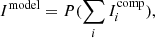
When processing data with a sufficiently small field of view a common practice is to ignore the effects of sky curvature and non-coplanar array, and so we can write the measurement equation as
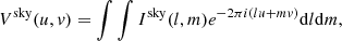
where (u, v) is the baseline coordinate and (l, m) is the coordinate in the tangent plane. Obviously, the visibility function Vsky(u, v) and the sky brightness distribution Isky(l, m) are a Fourier transform pair. In practical radio interferometry, incomplete spatial frequency sampling means the effects of the sampling function S(u, v) must be considered. Now the measured visibility Vobs(u, v) can be expressed as

Then we compute the observed image from the visibility domain by an inverse two-dimensional Fourier transform. Due to the small field of view, the distortion of the sources here is negligible. So we can use the deconvolution method to remove the effects of incomplete sampling to achieve effective modeling of the sky. However, next-generation telescope arrays such as the 21 CentiMeter Array (21CMA; Zheng et al. 2016), the Murchison Widefield Array (MWA; Tingay et al. 2013), the LOw Frequency ARray (LOFAR; van Haarlem et al. 2013), the Hydrogen Epoch of Reionization Array (HERA; DeBoer et al. 2017), and the SKA (Mellema et al. 2013; Wu 2019) have or will have wider fields of view. The effects of sky curvature and non-coplanar arrays can no longer be ignored. Except for the case where all the samples are in a plane (such as an east-west array) (Cornwell et al. 2005), visibilities must be measured theoretically and practically in three-dimensional space (u, v, w) containing the w-term,
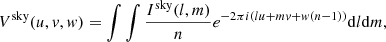
where 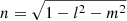 parameterizes the upper hemisphere and w represents this non-coplanar factor. If we ignore the effects of the w-term during wide-field imaging, it is difficult to accurately recover the sky signal. For example, the elimination of foreground bright sources is essential in EoR imaging. The w-term will cause distortion of the foreground sources far from the phase center of the image. These distortions make it extremely difficult to completely eliminate the effects of the foreground sources, so we cannot correctly reconstruct the EoR signals. This measurement equation containing the w-term allows us to find an optimal sky model from given wide-field measurement visibilities.
3. The Wide-field Imager
Obviously for a wide-field observation, it is no longer a two-dimensional Fourier relation between the data domain and image domain. During wide-field imaging, the effects of the w-term must be eliminated before reconstruction of the optimal sky model. In our imager, instead of some image-domain correction methods, we correct the w-term by using projection kernels in the uv domain. Here we rewrite the measurement equation as an integral form
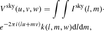
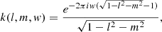
where k(l, m, w) is the w-term and ⋅ is the multiplicative operation. The exponential term of the w-term depends on the wavelength, aperture, and baseline. As the wavelength or baseline increases or the aperture decreases, the image degradation caused by the w-term will become more serious. The convolution theory states that the product of the image domain is a convolution in the Fourier domain. The measurement equation in the visibility domain is expressed as

where K(u, v, w) is the Fourier transform of k(l, m, w), the visibility function Vsky(u, v, w = 0) without the w-term is also a two-dimensional function, and * is a convolution operator. Now the three-dimensional function containing the effects of the w-term is a convolution of Vsky(u, v, w = 0) and K(u, v, w). K(u, v, w) can be recognized as the Fresnel diffraction of the electric field of one element sampling another element plane in a baseline. Therefore, this is a physical expression. Through this convolution function, the three-dimensional function Vsky(u, v, w) is a mapping of a two-dimensional plane. Here, a two-dimensional Fourier transform can be employed to achieve the transform from the image domain to the visibility domain. For a given sky brightness model, a two-dimensional Fourier transform is used to predict the sky model to the (u, v, w = 0) plane, and then the (u, v, w = 0) data is mapped to the measurement data points (u, v, w) by convolving with the w-projection function (Eq. (5)). The calculations here are limited to numerical errors. The error caused by applying this w-projection function during the process from visibilities to images can be eliminated by subsequent iterative operations, which are described in the following.
The w-projection method converts the three-dimensional measurement data into two-dimensional data. Then the observed/dirty image and dirty beam can be calculated by the inverse two-dimensional Fourier transform as follows (for the sake of discussion, we omit the coordinates and use the linear algebra representation):


Here F−1 represents the inverse two-dimensional Fourier transform; Iobs, Isky, Ipsf are the vectors of a dirty image, a sky brightness image, and a dirty beam, respectively; Vw is the two-dimensional visibilities transformed by the w-projection function; Ipsf is the inverse Fourier transform of the sampling matrix S; and B is a Toeplitz matrix with shifted row copies in Ipsf. The effects still need to be eliminated due to the degradation of the point spread function (PSF) caused by incomplete spatial frequency sampling and the errors caused by the previous calculations from the visibility domain to image domain.
The elimination of these effects essentially uses a PSF and an iterative approach to find emission components from the degraded dirty image. For sky reconstruction, the ability to model the sky plays an important role, which determines the quality of the reconstructed sky image. A very important factor is the scale parameter. In the scale-free and multi-scale sky models, the scale parameter becomes a key factor that restricts its representation ability. Even a multi-scale sky model is able to represent the correlation between neighboring pixels of the extended features and to construct a better sky image in the reconstruction of diffuse emission than a scale-free sky model. However, a multi-scale sky model is limited to a few enumerated scale sizes that cannot fit the uncertainty of the intrinsic scale of astrophysics targets. Therefore, an adaptive-scale sky model whose scale adaptively changes with the intrinsic scale of the sky emission is the essential requirement for the reconstruction of astrophysical targets (Bhatnagar & Cornwell 2004; Zhang 2018). In our imager we use explicit fitting to achieve consistency between the scale of the reconstructed model and the intrinsic scale of sky emission so that each model component is optimal. This requires minimizing the following objective function for each component in the minor cycle,
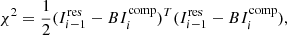
where  is the ith optimized component. The optimal scale is achieved by continuously updating the gradient,
![$$ \begin{aligned} \frac{\partial \chi ^{2}}{\partial p_{i}} = -\left[I_{i-1}^\mathrm{res}\right]^{T}\frac{\partial I_{i}^\mathrm{comp}}{\partial p_{i}}, \end{aligned} $$](/articles/aa/full_html/2020/08/aa38153-20/aa38153-20-eq12.gif)
where pi is the parameters from the component 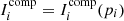 . Here
  is the residual image after eliminating the effects of the PSF of the i − 1th optimal model component, and is updated as
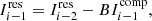
where  .
.
The initial values of these fitting parameters pi are found by a matched filtering method. In our imager, the estimation of the initial scale is no longer limited to a few specified scales; it uses the method of random scales, which we call the random-scale matched filtering method. Each initial fitting parameter is the best value selected from several random scales by finding the global peak from these images smoothed by these random scales. In order to quickly find the best component, the PSF is approximated as a Gaussian function so that we do not calculate convolution in the objective function (Eq. (9)). This random-scale method for estimating the initial parameters helps us to escape from the local optimum in this reconstruction process and to obtain a better model image.
When the residual peak value reaches the first sidelobe ratio of the PSF, the model image needs to be updated as
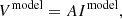
where P() is used to eliminate negative values of this model to get a non-negative model. This model then needs to be predicted on the measurement points to get the model visibilities,
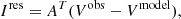
where A is actually the observation matrix. For a small field of view, A is approximated by OF, where F is a two-dimensional Fourier transform and O is usually a tapered prolate spheroidal wave function with a small support to achieve the projection of regular points to irregular measurement points. For wide-field imaging, A cannot use narrow field approximation due to the w-term. Instead A is approximated by WOF, where W is the w-projection, which is used to achieve accurate prediction of the w-term through Eq. (5). In fact, WO is first calculated as a convolution kernel and then to predict these regular points to measurement points. Then the residual image is updated as
and when Ires approaches noise or no longer changes, we obtain the optimal sky model. This essentially finds an optimal model that matches the observed data by minimizing

A smaller ϵ is generally considered to be a more consistent result with the original data.
In the imaging methods such as those presented by Bhatnagar et al. (2013) and Offringa et al. (2014), the wide-field effects of the w-term have been corrected, but they use the CLEAN-like scale-free or multi-scale model construction methods whose model construction ability is limited by fixed scale sizes. The existing CLEAN-like adaptive-scale model construction methods (Bhatnagar & Cornwell 2004; Zhang et al. 2016a,b; Zhang 2018) are only verified under the assumption of a small field of view. Our imager uses a newly proposed adaptive-scale model construction method, which is an optimal method based on random-scale matched filtering and positive constraints. It has the dual capabilities of the w-term correction and adaptive-scale model construction.
The scale adaptive ability through explicit fitting determines that our model scale is consistent with the intrinsic scale of the sky emission. Moreover, our imager guarantees the non-negativity of the model, which is in line with astrophysics. The w-projection models the w-phase term correctly. These factors determine that our imager can construct a physical adaptive-scale model with consistent sky brightness distribution and measurement data.
4. Results and discussion
4.1. Performance on simulated SKA data
In order to demonstrate the key motivation, the proposed imager is applied to SKA simulation data. The simulation of SKA observation1 is performed in the SKA1-LOW core configuration with the observation frequency at 100 megahertz. This uv sampling pattern is shown in Fig. 1, which has sufficient sampling between the shortest baseline and the longest baseline, which results in a nice PSF displayed in Fig. 2 middle. The reference image shown in Fig. 2 left is composed of the widely studied source M31 with medium complexity and two compact sources away from the phase center of the image. This dirty image degraded by the PSF is shown in Fig. 2 right. It can be seen that the sources are corrupted by the PSF and the two compact sources far away from the center of the image phase have produced relatively severe distortion. Our imager is used to correct these effects from the PSF and w-term distortion.
 |
Fig. 1. Uv coverage for the SKA simulation, recorded as seven snapshots whose time distribution is in [ − 3.0, −2.0, −1.0, 0.0, 1.0, 2.0, 3.0]*(π/12.0). |
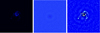 |
Fig. 2. Simulation results. Left: reference image with M 31 and two compact sources. Middle: PSF from the uv coverage (Fig. 1) is displayed with logarithmic scaling (CASA scaling power cycles = − 1.3) for more details. Right: Dirty image with w-term distortions. |
The reconstruction results of our imager are shown in Fig. 3. It can be seen that our imager can find a model image close to the reference image (Fig. 2 left). It is worth mentioning that the emission represented by our model image is positive, which is more in line with astrophysics. However, the model image (Fig. 4 left) obtained by the multi-scale method contains negative structures. The model error images (Fig. 5) shows that the model image reconstructed by our imager (Fig. 5 left) has less error than the reference image. This shows that our imager can reconstruct an image closer to the potential real sky brightness distribution. Compared to the dirty image, the source in our restored image (Fig. 3 right) already shows a clear structure; in particular, the non-source area no longer has a significant structure. This shows that the degradation caused by PSF has been completely eliminated. At the same time, the comparison found that the distortion of these compact sources far away from the center of the image phase has been significantly eliminated. These show that our imager has a good ability to reconstruct images with a large field of view.
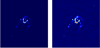 |
Fig. 3. Reconstruction results from our imager. Left: model image. Right: restored image. |
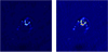 |
Fig. 4. Reconstruction results from w-projection and multi-scale CLEAN algorithms. Left: model image. Right: restored image. |
 |
Fig. 5. Model error images which are the difference between the model image and the reference image. Left: from our imager. Right: from w-projection and multi-scale CLEAN algorithms. The two model error images are displayed in the same data range and with the same logarithmic scaling (CASA scaling power cycles = − 1.5). |
Table 1 can confirm this conclusion. In this experiment, off-source root mean square (RMS) and RMS are significantly reduced, and the dynamic range of the restored image is also greatly improved because our imager uses an adaptive-scale sky model, which has a strong spatial scale construction capability, to obtain a better reconstruction.
Numerical comparison of different algorithms on simulated data for SKA observation.
In order to further verify our imager, the effects of the number of different scales on the total reconstructed flux are shown in Fig. 6. This shows that our imager can converge to the same level with different scale numbers. Several scales (e.g. 4–8) are typically required to find a good initial parameter values in other adaptive-scale algorithms, while our imager can use a scale to find suitable initial parameter values. It can be seen that our imager can obtain stable reconstruction results even at an initial scale. In addition, since we used a random-scale matched filtering method, Fig. 6 also shows that although different initial parameter values have an effect on the behavior of the model update, they can converge to the same level. The effects of the number of different scales on the RMS and off-source RMS displayed in Fig. 7 further confirm this conclusion.
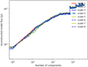 |
Fig. 6. Effects of the number of different scales on the total reconstructed flux. “scale N” indicates that N initial scales are used to search for the best initial scale. The total flux of the reference image is about 105.8 Jy and the reconstructed ratio is about 98.6%. |
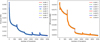 |
Fig. 7. Effects of the number of different scales on the RMS and off-source RMS. “scale N” indicates that N initial scales are used to search for the best initial scale. |
The effects of different noise levels on the total reconstructed flux are shown in Fig. 8, and the effects on the RMS and off-source RMS are displayed in Fig. 9. It can be seen that our imager can obtain stable reconstruction at a higher peak signal-to-noise ratio, which shows that our imager has a certain anti-noise performance. But when the peak signal-to-noise is relatively low, it will also limit the full reconstruction of the signal.
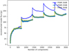 |
Fig. 8. Effects of different noise levels on the total reconstructed flux. |
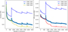 |
Fig. 9. Effects of different noise levels on the RMS and off-source RMS. |
Overall, these examples have shown the powerful performance of our imager. Below we show the performance of our imager on real observation data.
4.2. Performance on real observation data
Here the real JVLA observation data of the supernova remnant G55.7+34 (Bhatnagar et al. 2011) are used to demonstrate the performance of our imager. At the same time, we compare our imager with the Högbom and multi-scale algorithms (Högbom 1974; Cornwell 2008) based on the w-projection correction in the Common Astronomy Software Applications package (CASA2). The G55.7+34 observation covered the entire L-band with 1 − 2 gigahertz. Robust weighting is used to balance angular resolution and sensitivity of compact and extended emission. The primary beam is about 28 arcmin in diameter, and the entire imaging area is approximately 170.67 arcmin (see Fig. A.1).
The dirty image generated by our imager with the w-term correction is shown in Fig. A.1 left, while the dirty image created by the standard imager is displayed in Fig. A.1 right. The standard imager assumes a small field of view that ignores the w-term so that its effects remain in this dirty image (Fig. A.1 right). This effect can distort sources that are out of the phase center, and this distortion becomes more severe as the distance from the phase center increases. We can see the source distortion has become severe at the edges of the image (see Fig. A.1 right). At the top of Fig. A.1, two tightly separated compact sources have been severely distorted due to the effects of the w-term so that they appear to have other structures around them (see Fig. A.2 right). The compact source at the bottom left of Fig. A.1 is so severely distorted that the structure cannot be identified (Fig. A.3 right). However, our imager can model this w-term well, and the w-projection method is used to eliminate the distortion of compact and non-compact sources (see Figs. A.2 left and A.3 left).
The results reconstructed from our imager are shown in Fig. A.4. This sidelobe-free restored image is shown in Fig. A.4 middle; it is the sum of the final residuals and smooth model image (Fig. A.4 right), which is a convolution of the reconstructed model and the CLEAN beam. This shows that our imager has effectively eliminated the effect of PSF sidelobes in the dirty image and the source distortion caused by the wide field of view.
The smooth model image reconstructed by our imager is shown in Fig. A.5 left, while the image reconstructed without w-term correction using the adaptive-scale model construction method included in our imager is shown in Fig. A.5 right. It can be seen that our adaptive-scale model construction method can clearly reconstruct astrophysics features. We now focus on the two substructures discussed above. The tightly separated features are well separated in the reconstructed image in our imager (Fig. A.6 left). However, if we only use our adaptive-scale model construction method, it can well eliminate the effects of the PSF sidelobes, but it cannot eliminate the effects of the w-term (Fig. A.6 right). If we look at that compact structure (Fig. A.7), we reach the same conclusion. Therefore, if we only use the adaptive-scale model construction method, we still cannot eliminate the effects of the w-term. Once the w-term correction and the adaptive-scale model construction methods are combined, we can eliminate both the wide-field effects of the w-term and the effects of the PSF sidelobes so that the celestial features in a wide field of view can be reconstructed well.
To further verify our imager, we compared it with the w-projection + Högbom deconvolution and w-projection + multi-scale deconvolution methods implemented in the CASA. The Högbom and multi-scale algorithms are typical scale-free and multi-scale sky model construction methods, respectively. The smooth model images reconstructed by these methods are shown in Fig. A.8. Overall, the model images reconstructed by the w-projection + Högbom deconvolution and w-projection + multi-scale deconvolution methods contain negative features around the supernova remnant, while the model image reconstructed by our imager does not. The angular resolution is higher for the tightly separated souces reconstructed by our imager (Fig. A.9 left). The reconstruction of that compact source is shown in Fig. A.10. It can be seen that our imager can model this source better. This stems from the powerful ability of our imager to construct adaptive-scale models. This sky modeling ability is significantly stronger than that of scale-free and multi-scale sky models.
5. Summary
In this work we proposed a new imager with w-term correction and adaptive-scale model construction that can accurately reconstruct the complicated celestial features observed in a wide field of view. This is the first time that the w-term correction has been combined with a CLEAN-like adaptive-scale model construction method. The w-projection method can effectively model the wide-field factor w-term, and map three-dimensional visibilities to a two-dimensional plane. This eliminates the w-term distortion of sources away from the phase center. The adaptive-scale model construction method uses an explicit fitting technique to realize the scale adaptation of sky models. This allows our imager to reconstruct a model consistent with the intrinsic scale of sky emission, which is important to improve the fidelity of the reconstructed image. The adaptive-scale model eliminates the errors caused by the scale uncertainty of the sky emission in the scale-free and multi-scale sky models. At the same time, the reconstructed emission is limited to being positive in this adaptive-scale model, which allows us to obtain a more physical model. So our imager can effectively solve the reconstruction problem of wide-field observations. It may be an alternative for wide-field imaging. This work is a step forward toward the wide-field imaging of the SKA. In the future, we will explore the imaging capabilities of our imager in the low frequency array of the SKA.
This SKA observation is simulated by the Radio Astronomy Simulation, Calibration and Imaging Library (RASCIL), which is officially developed by the SKA organization. It can be found at https://developer.skatelescope.org/projects/sim-tools/en/latest/ or https://github.com/SKA-ScienceDataProcessor/rascil; this library is for radio interferometry calibration and imaging algorithms using Python and numpy.
https://casa.nrao.edu/; its main goal is to support the data post-processing requirements of next-generation radio astronomical telescopes.
Acknowledgments
We would like to thank the many people who have worked and are working on Python, CASA and RASCIL projects, which together has resulted in an excellent development and simulation environment. This work was partially supported by the National Key R&D Program of China (2018YFA0404602), the National Natural Science Foundation of China (NSFC, 11963003), the Guizhou Science & Technology Plan Project (Platform Talent No.[2017]5788), the Youth Science & Technology Talents Development Project of Guizhou Education Department (No.KY[2018]119,[2018]433]), Guizhou University Talent Research Fund (No.(2018)60), and “Light of West China” Programme (2017-XBQNXZ-A-008).
References
- An, T. 2019, Sci. Chin.-Phys. Mech. Astron., 62, 989531 [CrossRef] [Google Scholar]
- Bhatnagar, S., & Cornwell, T. J. 2004, A&A, 426, 747 [NASA ADS] [CrossRef] [EDP Sciences] [Google Scholar]
- Bhatnagar, S., Rau, U., Green, D. A., & Rupen, M. P. 2011, ApJ, 739, L20 [NASA ADS] [CrossRef] [Google Scholar]
- Bhatnagar, S., Rau, U., & Golap, K. 2013, ApJ, 770, 91 [NASA ADS] [CrossRef] [Google Scholar]
- Clark, B. G. 1980, A&A, 89, 377 [NASA ADS] [Google Scholar]
- Cornwell, T. J. 1983, A&A, 121, 281 [NASA ADS] [Google Scholar]
- Cornwell, T. J. 2008, IEEE J. Sel. Top. Signal Process., 2, 793 [Google Scholar]
- Cornwell, T. J. 2009, A&A, 500, 65 [NASA ADS] [CrossRef] [EDP Sciences] [Google Scholar]
- Cornwell, T. J., & Evans, K. F. 1985, A&A, 143, 77 [NASA ADS] [Google Scholar]
- Cornwell, T. J., & Perley, R. A. 1992, A&A, 261, 353 [NASA ADS] [Google Scholar]
- Cornwell, T. J., Braun, R., & Briggs, D. S. 1999, ASP Conf. Ser., 180, 151 [Google Scholar]
- Cornwell, T. J., Golap, K., & Bhatnagar, S. 2005, in Wide Field Imaging Problems in Radio Astronomy, (ICASSP’05), Proc. IEEE Int. Conf. Acoustics Speech Signal Process., 5, 861 [Google Scholar]
- Cornwell, T. J., Golap, K., & Bhatnagar, S. 2008, IEEE J. Sel. Top. Signal Process., 2, 647 [NASA ADS] [CrossRef] [Google Scholar]
- Cornwell, T. J., Voronkov, M. A., & Humphreys, B. 2012, in Image Reconstruction from Incomplete Data VII, (Bellingham: SPIE), Proc. SPIE Conf. Ser., 8500, 85000L [CrossRef] [Google Scholar]
- DeBoer, D. R., Parsons, A. R., Aguirre, J. E., et al. 2017, PASP, 129, 045001 [NASA ADS] [CrossRef] [Google Scholar]
- Högbom, J. A. 1974, A&AS, 15, 417 [Google Scholar]
- Humphreys, B., & Cornwell, T. J. 2011, SKA MEMO 132, Available at: https://www.skatelescope.org/uploaded/59116_132_Memo_Humphreys.pdf [Google Scholar]
- Koopmans, L., Pritchard, J., Mellema, G., et al. 2015, Advancing Astrophysics with the Square Kilometre Array (AASKA14) [Google Scholar]
- Lao, B., An, T., Yu, A., et al. 2019, Sci. Bull., 64, 586 [CrossRef] [Google Scholar]
- Li, F., Cornwell, T. J., & de Hoog, F. 2011, A&A, 528, A31 [NASA ADS] [CrossRef] [EDP Sciences] [Google Scholar]
- Li, W., Xu, H., Ma, Z., et al. 2019, MNRAS, 485, 2628 [CrossRef] [Google Scholar]
- Narayan, R., & Nityananda, R. 1986, ARA&A, 24, 127 [NASA ADS] [CrossRef] [Google Scholar]
- Mellema, G., Koopmans, L. V., Abdalla, F. A., et al. 2013, Exp. Astron., 36, 235 [CrossRef] [Google Scholar]
- Offringa, A. R., McKinley, B., Hurley-Walker, N., et al. 2014, MNRAS, 444, 606 [NASA ADS] [CrossRef] [Google Scholar]
- Pawsey, J. L., Payne-Scott, R., & McCready, L. L. 1946, Nature, 157, 158 [CrossRef] [Google Scholar]
- Perley, R. A. 1999, in Imaging in Radio Astronomy II, A Collection of Lectures from the Sixth NRAO/NMIMT Synthesis Imaging Summer School, eds. G. B. Taylor, C. L. Carilli, & R. A. Perley (San Francisco: Astron. Soc. Pac.), ASP Conf. Ser., 180, 383 [Google Scholar]
- Pratley, L., Johnston-Hollitt, M., & McEwen, J. D. 2019, ApJ, 874, 174 [CrossRef] [Google Scholar]
- Rau, U. 2010, Ph.D. Thesis, New Mexico Institute of Mining and Technology, Socorro, NM, USA [Google Scholar]
- Rau, U., & Cornwell, T. J. 2011, A&A, 532, A71 [NASA ADS] [CrossRef] [EDP Sciences] [Google Scholar]
- Ryle, M., & Vonberg, D. D. 1948, RSPSA, 193, 98 [Google Scholar]
- Sault, R., Bock, D.-J., & Duncan, A. 1999, A&A, 139, 387 [NASA ADS] [CrossRef] [EDP Sciences] [Google Scholar]
- Schwab, F. R. 1984, AJ, 89, 1067 [NASA ADS] [CrossRef] [Google Scholar]
- Tasse, C., van der Tol, S., van Zwieten, J., et al. 2013, A&A, 553, A105 [NASA ADS] [CrossRef] [EDP Sciences] [Google Scholar]
- Tingay, S. J., Goeke, R., Bowman, J. D., et al. 2013, PASP, 30, 7 [Google Scholar]
- Thompson, A. R., Moran, J. M., & Swenson, G. W. 2017, Interferometry and Synthesis in Radio Astronomy, 3rd edn. (Springer) [Google Scholar]
- van Haarlem, M. P., Wise, M. W., Gunst, A. W., et al. 2013, A&A, 556, A2 [NASA ADS] [CrossRef] [EDP Sciences] [Google Scholar]
- Wakin, M. 2008, IEEE Signal Proc. Mag., 21 [Google Scholar]
- Wu, X. P. 2019, China SKA Science Report (Science press) [Google Scholar]
- Zhang, L. 2018, A&A, 618, A117 [CrossRef] [EDP Sciences] [Google Scholar]
- Zhang, L., Bhatnagar, S., Rau U., & Zhang M. 2016a, A&A, 592, A128 [NASA ADS] [CrossRef] [EDP Sciences] [Google Scholar]
- Zhang, L., Zhang, M., & Liu, X. 2016b, Ap&SS, 361, 153 [NASA ADS] [CrossRef] [Google Scholar]
- Zhang, L., Xu, L., & Zhang, M. 2020, PASP, 132, 041001 [CrossRef] [Google Scholar]
- Zheng, Q., Wu, X. P., Johnston-Hollitt, M., Gu, J. H., & Xu, H. 2016, ApJ, 832, 190 [CrossRef] [Google Scholar]
Appendix A: Results of real observation data
In this appendix the results of the JVLA observation data from different imagers are provided. Please refer to Sect. 4.2 for more information.
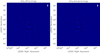 |
Fig. A.1. Dirty images from different imagers. Left: generated by our imager with w-term correction and peak flux of 6.165 mJy. Right: generated by a standard imager, which assumes a narrow imaging field of view, and peak flux of 6.147 mJy. |
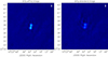 |
Fig. A.2. Tightly separated compact sources from the top of the imaging region in Fig. A.1. Left: from the dirty image generated by our imager with peak flux of 1.973 mJy. Right: from the dirty image generated by the standard imager with peak flux of 1.348 mJy. |
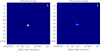 |
Fig. A.3. Compact source at the bottom left of Fig. A.1. Left: from the dirty image generated by our imager with peak flux of 3.637 mJy. Right: from the dirty image generated by the standard imager with peak flux of 1.541 mJy. |
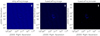 |
Fig. A.4. Results reconstructed from our imager. Left: dirty image with a w-term correction by the w-projection method and peak flux of 6.165 mJy. Middle: restored image whose PSF sidelobes have been eliminated and peak flux of 6.299 mJy. Right: smooth model image convolved with the CLEAN beam approximated from the PSF and peak flux of 6.153 mJy. |
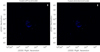 |
Fig. A.5. Model images convolved with the CLEAN beam approximated from the PSF. Left: reconstructed by our imager with peak flux of 6.153 mJy. Right: reconstructed by only our adaptive-scale model construct method included in our imager, but without the w-term correction and peak flux of 6.067 mJy. |
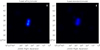 |
Fig. A.6. Tightly separated compact sources from the top of the imaging region in Fig. A.5. Left: reconstructed by our imager and peak flux of 1.979 mJy. Right: reconstructed by only our adaptive-scale model construct method included in our imager, but without the w-term correction and peak flux of 1.435 mJy. |
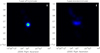 |
Fig. A.7. Compact source from the bottom left of the imaging region in Fig. A.5. Left: reconstructed by our imager and with peak flux of 3.464 mJy. Right: reconstructed by only our adaptive-scale model construct method included in our imager, but without the w-term correction and with peak flux of 1.556 mJy. |
 |
Fig. A.8. Smooth model images from different methods. Left: reconstructed by our imager with peak flux of 6.153 mJy. Middle: reconstructed by the w-projection + multi-scale deconvolution method implemented in the CASA and with peak flux of 6.154 mJy. Right: reconstructed by the w-projection + Högbom deconvolution method implemented in the CASA and with peak flux of 6.019 mJy. |
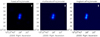 |
Fig. A.9. Tightly separated compact sources from the top of the imaging region in Fig. A.8. Left: reconstructed by our imager with the peak flux of 1.979 mJy. Middle: reconstructed by the w-projection + multi-scale deconvolution method implemented in the CASA and with peak flux of 1.980 mJy. Right: reconstructed by the w-projection + Högbom deconvolution method implemented in the CASA and with peak flux of 2.017 mJy. |
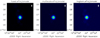 |
Fig. A.10. Compact source from the bottom left of the imaging region in Fig. A.8. Left: reconstructed by our imager with peak flux of 3.464 mJy. Middle: reconstructed by the w-projection + multi-scale deconvolution method implemented in the CASA and with peak flux of 3.524 mJy. Right: reconstructed by the w-projection + Högbom deconvolution method implemented in the CASA and with peak flux of 3.628 mJy. |
All Tables
Numerical comparison of different algorithms on simulated data for SKA observation.
All Figures
|
Fig. 1. Uv coverage for the SKA simulation, recorded as seven snapshots whose time distribution is in [ − 3.0, −2.0, −1.0, 0.0, 1.0, 2.0, 3.0]*(π/12.0). |
| In the text | |
|
Fig. 2. Simulation results. Left: reference image with M 31 and two compact sources. Middle: PSF from the uv coverage (Fig. 1) is displayed with logarithmic scaling (CASA scaling power cycles = − 1.3) for more details. Right: Dirty image with w-term distortions. |
| In the text | |
|
Fig. 3. Reconstruction results from our imager. Left: model image. Right: restored image. |
| In the text | |
|
Fig. 4. Reconstruction results from w-projection and multi-scale CLEAN algorithms. Left: model image. Right: restored image. |
| In the text | |
|
Fig. 5. Model error images which are the difference between the model image and the reference image. Left: from our imager. Right: from w-projection and multi-scale CLEAN algorithms. The two model error images are displayed in the same data range and with the same logarithmic scaling (CASA scaling power cycles = − 1.5). |
| In the text | |
|
Fig. 6. Effects of the number of different scales on the total reconstructed flux. “scale N” indicates that N initial scales are used to search for the best initial scale. The total flux of the reference image is about 105.8 Jy and the reconstructed ratio is about 98.6%. |
| In the text | |
|
Fig. 7. Effects of the number of different scales on the RMS and off-source RMS. “scale N” indicates that N initial scales are used to search for the best initial scale. |
| In the text | |
|
Fig. 8. Effects of different noise levels on the total reconstructed flux. |
| In the text | |
|
Fig. 9. Effects of different noise levels on the RMS and off-source RMS. |
| In the text | |
|
Fig. A.1. Dirty images from different imagers. Left: generated by our imager with w-term correction and peak flux of 6.165 mJy. Right: generated by a standard imager, which assumes a narrow imaging field of view, and peak flux of 6.147 mJy. |
| In the text | |
|
Fig. A.2. Tightly separated compact sources from the top of the imaging region in Fig. A.1. Left: from the dirty image generated by our imager with peak flux of 1.973 mJy. Right: from the dirty image generated by the standard imager with peak flux of 1.348 mJy. |
| In the text | |
|
Fig. A.3. Compact source at the bottom left of Fig. A.1. Left: from the dirty image generated by our imager with peak flux of 3.637 mJy. Right: from the dirty image generated by the standard imager with peak flux of 1.541 mJy. |
| In the text | |
|
Fig. A.4. Results reconstructed from our imager. Left: dirty image with a w-term correction by the w-projection method and peak flux of 6.165 mJy. Middle: restored image whose PSF sidelobes have been eliminated and peak flux of 6.299 mJy. Right: smooth model image convolved with the CLEAN beam approximated from the PSF and peak flux of 6.153 mJy. |
| In the text | |
|
Fig. A.5. Model images convolved with the CLEAN beam approximated from the PSF. Left: reconstructed by our imager with peak flux of 6.153 mJy. Right: reconstructed by only our adaptive-scale model construct method included in our imager, but without the w-term correction and peak flux of 6.067 mJy. |
| In the text | |
|
Fig. A.6. Tightly separated compact sources from the top of the imaging region in Fig. A.5. Left: reconstructed by our imager and peak flux of 1.979 mJy. Right: reconstructed by only our adaptive-scale model construct method included in our imager, but without the w-term correction and peak flux of 1.435 mJy. |
| In the text | |
|
Fig. A.7. Compact source from the bottom left of the imaging region in Fig. A.5. Left: reconstructed by our imager and with peak flux of 3.464 mJy. Right: reconstructed by only our adaptive-scale model construct method included in our imager, but without the w-term correction and with peak flux of 1.556 mJy. |
| In the text | |
|
Fig. A.8. Smooth model images from different methods. Left: reconstructed by our imager with peak flux of 6.153 mJy. Middle: reconstructed by the w-projection + multi-scale deconvolution method implemented in the CASA and with peak flux of 6.154 mJy. Right: reconstructed by the w-projection + Högbom deconvolution method implemented in the CASA and with peak flux of 6.019 mJy. |
| In the text | |
|
Fig. A.9. Tightly separated compact sources from the top of the imaging region in Fig. A.8. Left: reconstructed by our imager with the peak flux of 1.979 mJy. Middle: reconstructed by the w-projection + multi-scale deconvolution method implemented in the CASA and with peak flux of 1.980 mJy. Right: reconstructed by the w-projection + Högbom deconvolution method implemented in the CASA and with peak flux of 2.017 mJy. |
| In the text | |
|
Fig. A.10. Compact source from the bottom left of the imaging region in Fig. A.8. Left: reconstructed by our imager with peak flux of 3.464 mJy. Middle: reconstructed by the w-projection + multi-scale deconvolution method implemented in the CASA and with peak flux of 3.524 mJy. Right: reconstructed by the w-projection + Högbom deconvolution method implemented in the CASA and with peak flux of 3.628 mJy. |
| In the text | |
Current usage metrics show cumulative count of Article Views (full-text article views including HTML views, PDF and ePub downloads, according to the available data) and Abstracts Views on Vision4Press platform.
Data correspond to usage on the plateform after 2015. The current usage metrics is available 48-96 hours after online publication and is updated daily on week days.
Initial download of the metrics may take a while.