| Issue |
A&A
Volume 642, October 2020
|
|
|---|---|---|
| Article Number | A170 | |
| Number of page(s) | 9 | |
| Section | Planets and planetary systems | |
| DOI | https://doi.org/10.1051/0004-6361/201936897 | |
| Published online | 16 October 2020 | |
The residence-time of Jovian electrons in the inner heliosphere
1
Institut für Experimentelle und Angewandte Physik, Christian-Albrechts Universität zu Kiel,
Leibnizstraße 11,
24118
Kiel, Germany
e-mail: This email address is being protected from spambots. You need JavaScript enabled to view it.
2
Centre for Space Research, North-West University,
2520
Potchefstroom, South Africa
3
Theoretische Physik IV, Ruhr-Universität Bochum, Universitätsstr. 150,
44801
Bochum, Germany
Received:
11
October
2019
Accepted:
21
May
2020
Abstract
Context. Jovian electrons serve an important role in test-particle distribution in the inner heliosphere. They have been used extensively in the past to study the (diffusive) transport of cosmic rays in the inner heliosphere. With new limits on the Jovian source function, that is, the particle intensity just outside the Jovian magnetosphere, and a new set of in-situ observations at 1 AU for cases of both good and poor magnetic connection between the source and observer, we revisit some of these earlier simulations.
Aims. We aim to find the optimal numerical set-up that can be used to simulate the propagation of 6 MeV Jovian electrons in the inner heliosphere. Using such a setup, we further aim to study the residence (propagation) times of these particles for different levels of magnetic connection between Jupiter and an observer at Earth (1 AU).
Methods. Using an advanced Jovian electron propagation model based on the stochastic differential equation approach, we calculated the Jovian electron intensity for different model parameters. A comparison with observations leads to an optimal numerical setup, which was then used to calculate the so-called residence (propagation) times of these particles.
Results. Through a comparison with in-situ observations, we were able to derive transport parameters that are appropriate for the study of the propagation of 6 MeV Jovian electrons in the inner heliosphere. Moreover, using these values, we show that the method of calculating the residence time applied in the existing literature is not suited to being interpreted as the propagation time of physical particles. This is due to an incorrect weighting of the probability distribution. We applied a new method, where the results from each pseudo-particle are weighted by its resulting phase-space density (i.e. the number of physical particles that it represents). We thereby obtained more reliable estimates for the propagation time.
Key words: methods: numerical / Sun: heliosphere / diffusion / interplanetary medium / astroparticle physics / turbulence
© ESO 2020
1 Introduction
Over the last decade, solving particle transport equations by means of stochastic differential equation (SDEs) has become an increasingly popular tool due to increasing computational power. Whereas many of these studies are focused on galactic cosmic ray (GCRs), this work builds upon recent research regarding Jovian electrons (see Vogt et al. 2018; Nndanganeni & Potgieter 2018, and references therein). Since Jupiter is essentially a “steady state point source” of MeV electrons, Jovian electrons present a unique opportunity to study particle transport in the inner heliosphere. Detailed computational parameter studies have also become more feasible due to the enhanced computational capabilities acquired by utilising Nvidia’s Compute Unified Device Architecture (CUDA) as described by Dunzlaff et al. (2015). Here we study the residence time of energetic Jovians in the heliosphere (see e.g. McKibben et al. 2005, and references therein). Since Jupiter is assumed to release electrons continuously, these times are not directly measurable, and therefore have to be derived from theory or modelling. In order to develop a reliable estimation of the residence or propagation time, it is therefore necessary to (1) determine if the computational setup is realistic and to (2) validate the transport parameters against spacecraft data. This work will address both.
As for modulation studies of GCRs, an essential constraint for such an investigation is the knowledge of the source spectrum. The Jovian electron source spectrum was recently determined by Vogt et al. (2018) and is shown in Fig. 1. Knowledge of this spectrum allows us to estimate the effects of various physical parameters on computed Jovian intensities, which can also be compared to spacecraft observations of the same at Earth taken during periods of good and bad magnetic connection with the Jovian source. These comparisons can then provide insights with regard to the behaviour of quantities such as the low-energy electron diffusion coefficients parallel and perpendicular to the heliospheric magnetic field, as well as an optimised, realistic parameter set for further model computations as proposed in Table 2, which is used to study the residence times of Jovian electrons. We focussed our simulations on 6 MeV electrons during quiet-time conditions. This choice is in agreement with most prior investigations on Jovian electrons (see e.g. Kissmann et al. 2004; Nndanganeni & Potgieter 2018, and references therein) as it covers the detection range of several particle detection instruments such as Ulysses/KET, Voyager 1/TET, ISEE 3/ICE, IMP-8/CRNC, and SOHO/EPHIN.
In order to estimate the residence times, we propose a similar formalism as the one used to transform the probability densities resulting from the transport equation (TPE) into differential intensities. As this is done by a convolution with the source spectrum (see e.g. Strauss & Effenberger 2017, and references therein), an equivalent convolution is applied to the simulation times provided by the SDEs code. It has been demonstrated that the method of calculating residence times employed by, e.g., Florinski & Pogorelov (2009) and Strauss et al. (2013), cannot be interpreted as the propagation time of physical particles. We propose a novel approach in which the results from each pseudo-particle are weighted by its resulting phase-space density (i.e. the number of physical particles that it represents) to obtain estimates for the propagation time that are more consistent with the limited observational constraints, but also more representative of the propagation time of the physical particles themselves.
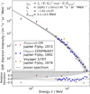 |
Fig. 1 Jovian source spectrum according to Vogt et al. (2018). Upper panel: source spectrum as fitted to the Pioneer 10 CPI and Ulysses COSPIN/KET data. The Voyager 1 TET data added in this plot appears to be in agreement as well. Lower panel: relative deviation of the spacecraft data from the fit. The shaded area covers the ± σ uncertainty. |
2 Scientific background
2.1 Jovian electrons as test particles
The scientific discussion of Jovian electrons dates back to the early 1970s when McDonald et al. (1972) proposed the existence of a dominant Jovian source by addressing the correlation of the ~ 13 month periodicity in low-MeV electron counting rate measurements at Earth orbit with Jupiter’s synodic period. Following the Jupiter flyby of Pioneer 10, Teegarden et al. (1974) were able to confirm this hypothesis based on data obtained by the Charged Particle Instrument (CPI). Pyle & Simpson (1977) showed through an analysis of the electron fluxes as a function of distance and their dependence on the occurrence of corotating interaction region (CIRs), that the Jovian source is not only quasi-continuous but also point-like. This refers to the observation that no electron emission could be detected from Jupiter’s magneto-tail, which extends up to over 1 AU into the heliosphere.
As the dominant particle population, from a few to several tens of MeV in the inner heliosphere, Jovian electrons soon became the subject of charged particle transport modelling (Conlon 1978; Zhang et al. 2017). Due to Jupiter’s decentralised position, the magnetic connection by means of the Parker spirals determines whether the electrons reach the observer primarily via motion along the field or by diffusion perpendicular to it. Thus, Jovian electrons are ideal candidates to probe the electron diffusion coefficients in the inner heliosphere.
Jovian electrons were used as test particles to model the charged-particle transport computationally (see e.g. Chenette et al. 1977; Conlon 1978; Fichtner et al. 2000; Zhang et al. 2007, and references therein) to ascertain the diffusion coefficients parallel and perpendicular to the Heliospheric Magnetic Field (HMF). This was usually done by comparing computed with measured electron intensities at Earth during periods of good or bad magnetic connection. Furthermore, given the demonstrated sensitivity of computed low-energy galactic electron intensities to various turbulence quantities (see Engelbrecht & Burger 2010, 2013; Engelbrecht 2019), it may be possible to draw conclusions from Jovian electrons to better understand the behaviour of those quantities in regions of the heliosphere where spacecraft observations of this character do not exist (see, e.g., Engelbrecht 2017). Since these transport parameters and the diffusion coefficients they depend on are spatially dependent, the time that particles reside in a certain part of the heliosphere may yield significant insights to the modulation of GCRs as well. Florinski & Pogorelov (2009) showed this dependency for GCR protons, investigating the time they spend in the heliotail, in the heliosheath, and in the solar wind within the termination shock, respectively. Utilising both galactic electrons and protons, Strauss et al. (2011a) focussed on the connection between thetotal propagation time and energy losses. They find a significant non-linear dependency on the total propagation times, which is strong enough to influence also the observations of Jovian electrons. These energy losses are entirely caused by adiabatic effects as other possible influences such as particle-particle interactions are negligible in the TPE due to a lack of significance in the interplanetary medium. As the adiabatic energy changes d E∕d t ~−2∕3 ⋅ EuSW∕r are connected to the radial position, the corresponding energy loss rate per step only depends on the temporal step size Δs and the radial position after the step. The radial direction of the step is thereby irrelevant. This leads to particles spending more simulation time at small radii losing more energy and implicitly to a statistical connection between the average energy losses and the particle’s mean free paths.
2.2 The Jovian electron spectrum
Parallel to the efforts of studying Jovian electron transport, the Jovian source itself has been investigated intensively. The main unknowns are the energy spectrum of the source and the way in which the particles are accelerated.
Source energy spectrum
Although it is widely considered to be dominant in its energy range, the shape and exact strength of the Jovian source remains a topic of debate. A preliminary suggestion was published as soon as Pioneer 10 confirmed the existence of the source by Teegarden et al. (1974), but the limited amount of flyby data and the general difficulties related to measuring electrons, especially electron spectra, made it difficult to further constrain both the magnitude and the shape. Suggestions were published by Baker & van Allen (1976), Eraker (1982), Haasbroek et al. (1997) and Ferreira et al. (2001) based on both Pioneer 10 CPI flyby and Earth orbit data. The two Voyagers and Ulysses are the only spacecraft equipped with particle instruments that could resolve the electron spectra above a few MeV (see Heber et al. 2005; Vogt et al. 2018; Nndanganeni & Potgieter 2018, and references therein). The latter two published source energy spectra jjov (E) shown in Fig. 1 on the basis of these flyby data. Vogt et al. (2018) proposed
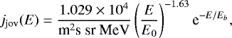 (1)
(1)
with E, and E0 the kinetic and rest energy of the electron, and Eb = 9.4 MeV the spectral break energy. The exponent of α = −1.63 is very much in agreement with the findings of Ferreira et al. (2001) and Baker & van Allen (1976), the shape proposed in Eq. (1) is more similar to that suggested by Teegarden et al. (1974) and Eraker (1982), and acceleration theory in itself, as Ferreira et al. (2001) proposed a combination of two spectra to fit the spectral break. The Voyager 1 flyby spectrum, as published by Nndanganeni & Potgieter (2018), is included in Fig. 1 and supports these results. An overview of the electron spectral data utilised for this study, obtained both during the flybys and at Earth’s orbit, is listed in Table 1. Previous studies derived the spectra by solving the particle transport equation and fitting the results to measurements close to Earth (see, for example Moses 1987, and references therein).
Overview of the electron spectra used in this study.
Acceleration processes
Since the findings of Bolton et al. (1989) were published, it has been widely accepted that Jovian electrons originate in the solar wind, then they are picked up by the Jovian magnetosphere and diffuse inwards. In situ data has been obtained by spacecraft such as Pioneer 10, Galileo, and Cassini and found to suggest acceleration via wave-particle interaction within the radiation belts, as discussed by Horne et al. (2008), alongside adiabatic processes suggested by de Pater & Goertz (1990). Because the existence of the Jovian source seems to be linked to the planet’s extended and strong magnetic field, the question as to whether these processes also apply close to Saturn is relevant as well (see e.g Lange & Fichtner 2008). Recently, Cassini measurements (as reported by Palmaerts et al. 2016; Roussos et al. 2016) revived this discussion and provide support, together with Galileo data, for the dominant role of adiabatic processes within both planets’ magnetospheres in order to accelerate MeV electrons (see Kollmann et al. 2018, and references therein).
Due to the recent measurements of electrons outside the heliosphere (Stone et al. 2013), the question of how to distinguish the Jovian population from the Galactic background, based on suggestions for the very local interstellar spectrum (VLIS) has been discussed in Bisschoff et al. (2019, and references therein). Apart from its implications regarding the modulation of GCRs, Nndanganeni & Potgieter (2018) find the Jovian population dominating the spectrum up to energies of about E ~ 25 MeV, followed by an energy range of 25 MeV ≤ E ≤ 40 MeV where the spectrum consists of a mixture of Jovian and Galactic electrons varied by the co-longitudinal dependency of the Jovian intensities. Regarding the radial dependency, Jovian electrons were found to be the dominant populations up to radial distances of R ~ 15 AU, based on simulations of the 6 MeV Jovian and Galactic electron intensities.
3 Calculating differential intensities
For the purpose of this study, the SDE code as discussed by Dunzlaff et al. (2009) was utilised, which is based on previous codes by e.g. Strauss et al. (2011b,a). This SDE solver is written in CUDA to optimise on performance time, and therefore incorporates a simplified analytical approach for both the solar wind velocity as well as for the HMF. The solar wind velocity is chosen to be uSW= 400 km s−1 and directed radially outwards. The HMF is assumed to be Parker-like and included geometrically within the diffusion tensor according to Burger et al. (2000). Therefore, the results of this study are applicable to solar minimum conditions.
It has been established, based on models (e.g. Potgieter 1996; Burger et al. 2000; Ferreira & Potgieter 2002) as well as from a theoretical perspective (e.g. Bieber et al. 1994; Engelbrecht & Burger 2010) that drift effects can be neglected when studying the transport of electrons with energies of a few MeV. In order to optimise the performance time of the code, the energy-independent approach of Dunzlaff et al. (2015) and Strauss et al. (2011b) is used to include the parallel and perpendicular mean free paths: λ∥ is normalised to a value of the parallel mean free path λ0 at 1 AU, such that:
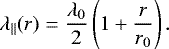 (2)
(2)
This value of the parallel mean free path, together with the particle speed ν, scales the parallel diffusion coefficient as κ∥(r) = νλ∥(r)∕3 and the perpendicular diffusion coefficient via the proportional factor χ such that:
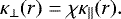 (3)
(3)
Although the above expressions represent an essentially ad hoc approach to modelling diffusion parameters, the radial dependency of the parallel diffusion coefficient does reproduce the corresponding behaviour of the quasi-linear theory electron parallel diffusion coefficient employed by Engelbrecht & Burger (2013), between 1 and 5 AU. Perpendicular mean free path expressions from theory, however, can behave in a manner quite different from what is assumed in this study (see, e.g. Shalchi 2009; Engelbrecht & Burger 2015; Gammon & Shalchi 2017). For a preliminary study, however, the above expression for κ⊥ should provide a reasonable approximation that meets the requirements for the scientific tasks investigated herein. This assumption is confirmed later within this study as the approach leads to reasonable results for the limited energy range considered.
As described in great detail by e.g. Kloeden & Platen (2011), the stochastic nature of diffusion is treated within the SDE method as a Wiener process  with ζ being a vector of Gaussian distributed random numbers. The resulting set of four integral equations, as they are derived by Strauss et al. (2011b), is solved iteratively by applying the Euler-Maruyama scheme. This leads to a random walk type solution which is terminated if a spatial or temporal boundary is reached, as shown in Fig. 2 for various possible exit positions. A time-backward phase-space trajectory can either terminate at the assumed position of the heliopause (blue line), the Jovian magnetosphere (orange line), or after a pre-specified number of steps have been made without an encounter with either of the formerly mentioned structures (green line). As discussed in Sect. 2.2, in the low-MeV energy range Jovian electrons dominate the spectrum. The solar population therefore can be assumed to be negligible during quiettimes, and thus trajectories exiting at the Sun are discarded. Galactic electrons, on the other hand are considered via the local interstellar spectrum according to Potgieter & Vos (2017), although the transport of the Galactic population into the inner heliosphere is much more sensitive to the drift effect, which is not considered here.
Instead of solving Parker’s TPE directly to obtain a time-dependent distribution function f(r, t) covering thewhole phase space, the SDE method provides a chain of point-like solutions both in space and time. The solutions must be sampled at a large number of phase-space points to approximate a spatial solution covering the phase space of interest. In order for the computational results to be comparable with spacecraft data, the time-backward setup is solved as derived and discussed by e.g. Kopp et al. (2012). A comparison between the time-forward and time-backward setup, made using a simpler 1D model, can be found in the review by Strauss & Effenberger (2017).
The left panel of Fig. 5 shows histograms of the so called exit energy1 (i.e. the energy of which pseudo-particles leave the computational domain) at times of good magnetic connection between the Jovian magnetosphere and the observational point, in contrast to Fig. 5b, which illustrates the energy distribution for an observational point in opposition to the Jovian source. The distributions in Fig. 5b are much broader. This, of course, is in agreement with Fig. 5a being dominated by the much more efficient parallel diffusion along the nominal Parker spirals, while pseudo-particles reaching the Jovian magnetosphere in Fig. 5b must do so via the more inefficient perpendicular diffusion process. These particles suffer much more scattering, leading to a more diffuse distribution.
Taking the integral distributions (dashed lines) into account, it shows that these extreme particle trajectories corresponding to high exit energies contribute very little to the total differential intensity. In the case of good connection, Fig. 5a suggest that the pseudo-particles with exit energies below 10 MeV contribute about 90% to the total differential intensity, whereas Fig. 5b shows that in the case of bad connection, they still make up about 80%. Therefore, we conclude that although the trajectory of each pseudo-particle is (mathematically) equally likely, they do not contribute equally towards the differential intensity. This is equivalent to stating that different pseudo-particles represent different amounts of physical particles corresponding to their physical significance.
The concern is now to consider that if each pseudo-particle represents a different number of real particles, is it necessary to weigh the pseudo-particles equally when calculating physical quantities, such as the residence time, from their distribution.
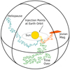 |
Fig. 2 Sketch of the simulation setup as detailed in Dunzlaff et al. (2015). The four different exit possibilities are colour-coded: the Sun (yellow), the Jovian magnetosphere (orange), the Heliopause (blue), as well as the option that the phase space trajectory is terminated by reaching a predefined end time (green). We note that the figure is not to scale. |
3.1 Model parameter dependencies
A major aspect of modelling physical processes is simplifying the computational setup in order to save resources and time without affecting the physical validity of the results. Therefore, the variability of our results was tested against various model setups in order to find the most optimal modelling scenario.
The choice of time increment Δs has the most obvious influence on the simulation results due to its association with the Wiener process and, hence, with the mathematical representation of diffusion. Both the effects of the size of the time increments and the influence of the maximal simulation time have been tested. For Δs a high sensitivity to the magnetic connection was observed as expected since the time increment (which is related to the adiabatic energy changes) influences the duration of the random walk. Therefore, it is important to note that the effect is more significant for observation points of good magnetic connections. As the trajectories for bad connections are much more diffusion-dominated, the effect of the size of the time increment is more likely to be cancelled out by the number of timesteps. For good connections, however, the trajectories are much more dominated by the geometry of the underlying HMF. Therefore, larger time increments cause larger abbreviations and subsequently longer simulation times. It was found that the simulated differential intensity converges for values of Δs ≤ 0.001 in programme units (about 0.004 days). The numerical dependence on the maximal duration of simulation appears to be very weak (above a certain limit), with a required duration of about 700 to 800 programm units in order to avoid deviations ofmore than 20. This leads to a total time of simulations of ∑ Δs ≥ 300 days. As the numerical step sizes of the pseudo-particles are ultimately dependent on the choice of the energy transport parameters (which influences the diffusive step size), there is a slight energy dependence on the optimal size of the timestep.
Due to the fact that Jovian electrons originate in and populate mainly the inner heliosphere, it seems natural to raise the question as to whether a model heliosphere could be restricted in size so that calculation results remain unaffected. It was found that results become insensitive to the size of the model heliosphere if RHP≥ 80 AU is used. For smaller radii, the resulting differential intensities increase exponentially, regardless of magnetic connection. Therefore, we use a value of RHP = 120 AU in order to assure convergence, and, as reported by e.g. Gurnett et al. (2013), this is the radial distance at which Voyager 1 crossed the heliopause.
A more physical question is whether a co-rotating coordinate system is necessary. To keep the setup mathematically as simple as possible, the code is designed in a way that both the Sun and the Jovian source are kept fixed. The position of the observer as the starting point of the time-backward phase space trajectories is calculated in a coordinate system relative to the slow orbital motion of Jupiter. These relative position can be kept static during the random walk or include the further co-rotation of the Jovian source by means of an additional longitudinal advection velocity Vϕ = ΩSun ⋅ r. Figure 3 shows the calculated Jovian electron intensities, at Earth, for different energies as a function of longitude. Simulations were performed for both a co-rotating coordinate system (top panel) and for the case of a static Jupiter (bottom panel). The bottom panel shows the ratio of these two scenarios and proves that the ratio between the differential intensities for a co-rotating and a static approach appears to be significant. We conclude that Jovian co-rotation must be included in the model to produce reasonable results. We also conclude that the co-rotation of the Jovian source is an important effect that should be incorporated into the numerical model.
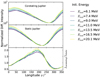 |
Fig. 3 Differential intensities of Jovian electrons for different initial energies Einit. Top panel: longitudinal variation due to varying connection for a co-rotating Jovian source, middle panel: case of a static Jupiter. Bottom panel: ratio of the results of the two approaches. |
3.2 Deriving an estimation for the mean free paths
Figure 5 shows that only lower-energy pseudo particles (with exit energies near the initial energy) contribute significantly to particle intensity at Earth. As this energy range only covers an order of magnitude, the energy dependence of the mean free paths both parallel and perpendicular can be neglected for the means of this study. We note, however, that the resulting diffusion coefficients, which are the parameters used in the model, might still have some energy dependence due to their dependence on the particle speed ν.
Thus, to estimate λ0, the Jovian spectral data at Earth orbit as listed in Table 1 were compared to the results of a parameter study covering the parameter space in question, namely λ∥ and λ⊥. As already discussed in Sect. 2.1, the decentralised position of the Jovian source allows us to estimate the effectiveness of parallel and perpendicular transport dependent on the observational point’s magnetic connection with Jupiter. In order to ensure consistency, λ∥ was determined when investigating the case of the best magnetic connection between the observational point and the source before determining χ which scales λ⊥ with respectto λ∥ according toEq. (3) and this, therefore, dominates the results in case of magnetic opposition.
The upper panel of Fig. 4a shows the available Jovian electron spectral data at Earth orbit during times of good magnetic connection. For a more detailed discussion with regards to the Jovian source spectrum, see Vogt et al. (2018) or the individual publications listed in Table 1. The black dashed line marks the shape of the Jovian source as fitted to the Earth orbit data in order to have a measure to define the deviation. The results of the simulations are colour-coded in all three panels, with varying parallel mean free paths covering the range of λ∥ = [0.05 AU, 0.4 AU] in steps of 0.05 AU, and a value of χ = 0.01 in agreement with the suggestions by Palmer (1982) as well as Bieber et al. (1994) and succesfully implemented in previous studies by (e.g. Strauss et al. 2011a; Vogt et al. 2018, amongst others) is used. The results are shown in the two upper panels of Fig. 4a; the top panel depicting the simulated intensities, whereas the middle panel shows their relative deviation from the nominal spectrum provided by the fit. The grey area marks the range of a ± 0.5 relative deviation in order to give an impression on the reliability of the results. As the errors related to the data appeared to be too small to be significant and it is way beyond the scope of this work to re-examine them, the choice was made to display the simulation results with respect to their relative deviation from the fit. In the bottom panel, the area between the lowest and the highest value of λ∥, leading to simulation results within this ± 0.5 relative deviation, is again marked in grey. Thereby it provides an estimation of the energy dependency of λ∥∕⊥. The energy range is chosen in order to cover the range of exit energies contributing to the total differential intensity for an inititial energy of 6 MeV according to Fig. 5. As it appears, a value of λ∥ = 0.15 AU seems to match the observations best over the whole energy range investigated herein. This is an additional motivation for our choice of an energy-independent mean free path.
Figure 4b shows the relative deviation of simulations with varying χ = [0.00, 0.04] and for two values for λ∥ = [0.125, 0.15] AU. The uppermost panel of Fig. 4b shows the spectral data at Earth’s orbit according to Table 1, specifically obtained during times of bad magnetic connection between the spacecraft and the Jovian magnetosphere. Similarly to Fig. 4a, the dashed line indicates the spectral shape of the source when fitted to the Earth orbit data. In this case the data are presumably dominated by the effects of perpendicular diffusion. As discussed above, larger values of λ∥ lead to more effective diffusion and, therefore, to increased differential intensities at the observational point. This relation is also present in the results depicted by Fig. 4b, as higher values of λ∥ demand smaller values of χ in order to fit the data. Although the estimation of parallel and perpendicular mean free paths based on turbulence theory is still an ongoing topic of research, previous studies suggest values between 0.09 and 0.3 AU for λ∥ (Palmer 1982; Bieber et al. 1994) which were tested successfully for electrons in the inner heliosphere such by studies such as, for example, Ferreira et al. (2003), Ferreira (2005), Strauss et al. (2011b) and Dröge et al. (2016) amongst others. While values of just λ∥ = 0.175 AU would would fit well within this range, they would demand values for χ that would be out of a realistic range (see e.g. Palmer 1982; Bieber et al. 1994; Strauss et al. 2011b; Dröge et al. 2016, amongst others) and, therefore, are considered unrealistic.
Taking the best fit χ for λ∥ = 0.15 AU (as the best-fitting value for λ∥ according to Fig. 4a) into account, a value of χ = 0.0125 seems to be justifiable within the margin of error for the energy range of interest. This value for the parallel mean free path is well within the Palmer (1982) consensus range, and reasonable for low-energy electrons (e.g. Bieber et al. 1994). The value for χ is somewhat smaller than the range expected from Palmer (1982), where 0.02 ≤ χ ≤ 0.08, but well within the range of values commonly used in numerical modulation studies (see, e.g. Ferreira et al. 2001; Engelbrecht & Burger 2013; Nndanganeni & Potgieter 2018). Therefore, unless otherwise indicated, these parameters were utilised throughout this study, as summarised in Table 2.
 |
Fig. 4 Simulated Jovian electron spectra used to optimize the values of λ∥ and χ. Top panel:a data fit (dashed line) along with the simulations results and spacecraft data obtained during corresponding time periods at the longitudinal point of best effective magnetic connection for different values of λ∥ = [0.05, 0.4] AU. Panel b does not show the simulated spectra for different values of for different values of χ = [0.005, 0.045] in the upper panel as the simulations are performed utilizing two different values for λ∥. The fit (dashed line) was performed utilizing spacecraft data by ISEE 3, the only spectral data formagnetically poorly connected observation times as given by Table 1. Lower panels: corresponding relative deviations from the fit (dashed lines) together with the ± 0.5 deviation area given in shaded grey and the spacecraft data. Lowest panel: shaded area marks the range of values for λ∥∕⊥ within the margin of less than ± 0.5 relative deviation. |
3.3 Interpretation of phase space trajectories
As already pointed out above, the phase space trajectories obtained by the SDE solver are mathematical solutions and, in contrast to a physical interpretation, each phase space trajectory is equally probable. However, not each phase space trajectory represents the same number of physical particles. Although they are often referred to as pseudo-particles, this term is slightly misleading because the phase space trajectories represent the evolution of the particle density distribution f along a curve through the heliosphere and has no connection with the trajectory of actual charged particles in a turbulent plasma.
The TPE is solved by integrating the SDEs via the time-backward Euler-Maruyama scheme which leads to an increase of the pseudo-particle’s energy Ei due to the inverse adiabatic processes (adiabatic energy losses treated in a time-backwards fashion). Therefore, applying the source spectrum jjov(E) as the boundary weight (see, e.g., Strauss et al. 2011b; Kopp et al. 2012) leads to the expression
 (4)
(4)
with the distribution function f as the solution of the TPE related to the differential intensity j = P2f, with P = pc∕q being the particle rigidity, depending on the momentum p and the charge q.
Equation (4) can also be derived by calculating the Green’s function G(xi, s = T) for any given boundary or initial condition in order to solve the convolution (see, e.g. Pei et al. 2010)
 (5)
(5)
with fb(x′, t) denoting the boundary value. As discussed by Strauss & Effenberger (2017), neglecting the initial condition simplifies Eq. (5) to
 (6)
(6)
with x = (r, E), fb (x, t) representingthe boundary condition (i.e. the particle population’s source distribution), ρ(x, t) being the conditional probability density and f(x0, t0) the distribution at the observational point. Focusing on steady state solutions where t → ∞⇒ ρ(xi, t) :→ ρ(xi), as well as calculating fi (x0, t0) for each phase space trajectory, ρi, individuallyreducing the spatial boundary of the integration domain Ωb to the exit position, rexit, as well as the range of the energy coordinates to Eexit then leads to the expression given by Eq. (4).
Figure 5 shows the probability density (binned distribution of pseudo-particles, Ni ∕N; red) and the elements of Eq. (4) ( ; blue) for an initialenergy of E0 = 6 Mev at an observational point at Earth. Whereas each pseudo-particle is equally weighted in the calculation, they may contribute very differently to the total differential intensity; from the figure, it is evident that pseudo-particles may reach the Jovian magnetosphere with several tens of MeV (which implies significant energy loss in the normal time-forward scenario). However, the blue histogram hints that only pseudo-particles with up to 10 MeV contribute significantly to the total differential intensity. The integral distributions (dashed line) for both cases further support this assumption as they converge roughly at the exit energies for which the fractional contribution of the differential intensity gets lower than the fractional contribution of pseudo-particles. Looking at just the distribution of the pseudo-particles may, therefore, prove misleading if we are interested in deriving physical quantities from the SDE method. It is important to note that even if some pseudo-particles contribute very little to the differential intensity, they cannot be disregarded in the calculations as they still contribute to the denominator of Eq. (4).
Computational and physical parameters used for the code (when not stated otherwise).
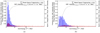 |
Fig. 5 Binned distributions of the exit energies |


4 Residence times
Because theEuler-Maruyama-Scheme (as well as alternative methods) utilises a well-defined time increment, ds, in order to solve for the system of integral equations, it is possible to derive a measure of τ as the time that the phase space trajectory takes to connect the source to the observational point. Thereby τ is calculated as the number of time steps needed for the phase space trajectory ni multiplied by the time increment d s, if the latter time step is assumed to be constant. Generally, τ can be givenas  , with
  and
and  often being simply the start time of the calculation. Although τi is often referred to as the propagation time or as the residence time too, the more accurate description would be to call τi the trajectory duration or simulation time.
This estimation raises the question of how to interpret the individual phase space trajectories. As discussed in Sect. 3, phase space trajectories are equally mathematically possible but not equally physically significant. If we now want toderive physical quantities from these trajectories, how should we weigh the resulting distributions? We aim to address this question in the next paragraphs.
Traditionally, the residence or propagation time is assumed to be equivalent to the expectation value of the time, as weighed by a probability density ρ,
 (7)
(7)
Typically, in previous works, ρ is constructed from the SDE solutions as the (normalised) distribution of the pseudo-particles’ exit time (see e.g. Florinski & Pogorelov 2009; Strauss et al. 2013). For 6 MeV Jovian electrons, these distributions are shown in Fig. 6, as the red histogram, for the case of good (left) and bad (right) magnetic connection to the source. From the red distribution, a propagation time of ~ 550−600 days is calculated, and from the figure itself, we note that most pseudo-particles only reach the observer within ~ 100−1000 days. This seems very long for relativistic electrons diffusing only a radial distance of ~ 4 AU towards Earth.
An observational estimate to compare with is discussed by Strauss et al. (2013). Investigating quiet-time increases (QTIs) (see e. g. McDonald et al. 1972; Chenette 1980), which relate to a diffusion barrier between Earth and Jupiter, these authors find that it takes ≈ 5 days after the diffusion barrier has passed Jupiter for the Jovian electrons to be detected again.
The numerical definition of τ according to Eq. (7) essentially weighs each pseudo-particle with the same probability. However, we have already seen earlier in this paper that each pseudo-particle does not represent the same number of physical particles. We therefore propose to rather use the distribution of particle density to calculate the propagation time by specifying
 (8)
(8)
which is normalised by the total phase-space density,
 (9)
(9)
Therebyf(x, t) represents the solution of the TPE and is calculated at the exit position xexit of the random walk. We note that f0(xexit) cancels in the calculation of τ, which in discrete form is read as:
 (10)
(10)
and s is the exit (integration) time of the pseudo-particles. Using this new definition, their weighted contribution to the propagation times are shown in Fig. 6 as the blue distribution. The parameters used for this simulation are listed in Table 2, as discussed in Sect. 3.2. These weighted propagation times are generally much shorter than those obtained by weighing the pseudo-particles equally. Similar values as the ones found by this study were only obtained using larger mean free paths (compare to e.g. Strauss et al. 2013) which would turn out to be unrealistic, as discussed in Sect. 3.2, because our findings are in agreement with prior studies on electron mean free paths such as (e.g. Palmer 1982; Bieber et al. 1994; Tautz & Shalchi 2013, amongst others) and modelling approaches by (e.g. Potgieter & Ferreira 2002; Dröge 2005; Strauss et al. 2011b, amongst others). By integrating the blue histograms, we find propagation times of ~ 5−11 days, almost two orders of magnitude shorter than the traditional calculation. Again, the comparison with the red histogram showing the pseudo-particle trajectories’ exit times makes this difference comprehensible. The integral distribution of the blue histograms (dashed lines) illustrate that the maximum of the exit times distribution (red) is almost a magnitude higher than the range of convergence. Normalised to the value of the residence time, the integral distributions (as for the differential intensities that are shown in Fig. 3) illustrate how little long exit times corresponding to large exit energies influence the residence times if calculated via Eq. (10). This leads to the disparity between the averaged exit or simulation times and our estimations of the residence time equivalent to the differences between the two distributions.
As we have shown and discussed in Sect. 3.3, this is caused by the diverging physical significance of the phase space trajectories. As Eq. (10) addresses and solves this problem, we consider our new calculation to be more representative of the propagation time of a physical particle. This is supported by the fact that Eq. (10) considers the exit or simulation times according to their representation of physical particles and therefore provides a measure consistent with the total differential intensity.
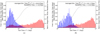 |
Fig. 6 Binned distributions of the Jovian electron propagation time using the normal (red) and new (blue) way of defining the probability distribution. Thereby panel a shows the distribution of exit times of pseudo-particles for a good magnetic connection between the observational point and the Jovian source and panel b for the case of poor magnetic connection. The blue distribution shows the weighted exit times, which we refer to as the propagation (residence) time of Jovian electrons. Again the integral distribution of the pseudo-trajectories contribution to τ is shown by the dashed line. The residence times are obtained via Eq. (10). |
5 Discussion and conclusions
In this paper, we discuss a Jovian electron transport model that is used to study the propagation times (residence times) of 6 MeV electrons. We discuss the optimal numerical set-up, including the choice of time step, integration times, and the required size of the numerical domain. We also show that taking into account the co-rotation of the Jovian source leads to non-negligible effects. Thisis an important effect due to its influence on the finite propagation time of Jovian particles from the observer (assumed at Earth, but at different longitudes) to the source. Figure 7 shows how the calculation of, for example, the propagation time, changes due to the assumption of either a static, or a co-rotating source.
We have also used the unique magnetic geometry of the Jovian propagation problem to quantify the appropriate mean free paths. By reproducing the 1 AU intensity spectrum during times of good magnetic connection, we were able to show that λ|| ≈ 0.1 AU is appropriate for Jovian electrons in the energy range under consideration. By doing the same during times of bad magnetic connection, we were able to show that a value of χ ≈ 0.01 is appropriate. Both these values fall within the range of what is expected from previous studies.
Using the optimal numerical set-up, we calculated the exit times of 6 MeV electrons using the traditional SDE formalism, where each pseudo-particle contributes equally to the final results. A value of ~ 600 days was found, which, while formally correct, does not seem physically consistent with relativistic particle propagating across a distance of ~ 4 AU. Therefore, we propose a new technique to weigh the resulting exit times with the particle intensity, leading to more realistic values of ~ 6 days. We propose to term these weighted exit times as the propagation (residence) time of Jovian electrons. The motivation for this weighing is as follows: although the trajectory of each pseudo-particle is equally probable, each pseudo-particle does not represent the same number of actual particles since the phase-space density of each pseudo-particle is different.
In the case of CIRs in particular, a more realistic measure of Jovian residence times could improve our understanding. As Jovian electron simulations successfully have been applied to this topic by Kissmann et al. (2003, 2004) the numerical set-up provided by this study provides the opportunity to revisit this approach with further insights. Simulations of residence times could also help to determine how much time Jovian electrons (and other particle populations) spend within structures like CIRs or magnetic flux tubes. More recently, Daibog et al. (2013) highlighted the role of Jovian electrons as test particles within this matter again, suggesting that deviations from their quiet time variations could serve as probes for the inner heliosphere’s structure.
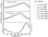 |
Fig. 7 Similarly to Fig. 3, the residence times (τ) of Jovian electrons are now shown in order to illustrate the influence of co-rotation of the Jovian source as compared to a static source. Bottom panel: ratio of the solutions. Different colours indicate different energies. |
Acknowledgements
This work is based on the research supported in part by the National Research Foundation of South Africa (Grant Number 111731) and the Deutsche Forschungsgemeinschaft (Grant Number FI 706/14). Opinions expressed and conclusions arrived at are those of the author and are not necessarily to be attributed to the NRF or DFG, respectively.
References
- Baker, D. N., & van Allen, J. A. 1976, J. Geophys. Res., 81, 617 [NASA ADS] [CrossRef] [Google Scholar]
- Bieber, J. W., Matthaeus, W. H., Smith, C. W., et al. 1994, ApJ, 420, 294 [Google Scholar]
- Bisschoff, D., Potgieter, M. S., & Aslam, O. P. M. 2019, ApJ, 878, 59 [CrossRef] [Google Scholar]
- Bolton, S. J., Gulkis, S., Klein, M. J., de Pater, I., & Thompson, T. J. 1989, J. Geophys. Res., 94, 121 [NASA ADS] [CrossRef] [Google Scholar]
- Burger, R. A., Potgieter, M. S., & Heber, B. 2000, J. Geophys. Res., 105, 27447 [Google Scholar]
- Chenette, D. L. 1980, J. Geophys. Res., 85, 2243 [NASA ADS] [CrossRef] [Google Scholar]
- Chenette, D. L., Conlon, T. F., Pyle, K. R., & Simpson, J. A. 1977, ApJ, 215, L95 [Google Scholar]
- Conlon, T. F. 1978, J. Geophys. Res., 83, 541 [NASA ADS] [CrossRef] [Google Scholar]
- Daibog, E. I., Kecskemety, K., & Logachev, Y. I. 2013, Bull. Russ. Acad. Sci. Phys., 77, 551 [CrossRef] [Google Scholar]
- de Pater, I., & Goertz, C. K. 1990, J. Geophys. Res., 95, 39 [NASA ADS] [CrossRef] [Google Scholar]
- Dröge, W. 2005, Adv. Space Res., 35, 532 [NASA ADS] [CrossRef] [Google Scholar]
- Dröge, W., Kartavykh, Y. Y., Dresing, N., & Klassen, A. 2016, ApJ, 826, 134 [NASA ADS] [CrossRef] [Google Scholar]
- Dunzlaff, P., Kopp, A., Heber, B., & Sternal, O. 2009, Proceedings of the 31st International Cosmic Ray Conference (ICRC) 2009 [Google Scholar]
- Dunzlaff, P., Strauss, R. D., & Potgieter, M. S. 2015, Comput. Phys. Commun., 192, 156 [NASA ADS] [CrossRef] [Google Scholar]
- Engelbrecht, N. E. 2017, ApJ, 849, L15 [CrossRef] [Google Scholar]
- Engelbrecht, N. E. 2019, ApJ, 872, 124 [CrossRef] [Google Scholar]
- Engelbrecht, N. E., & Burger, R. A. 2010, Adv. Space Res., 45, 1015 [CrossRef] [Google Scholar]
- Engelbrecht, N. E., & Burger, R. A. 2013, ApJ, 779, 158 [NASA ADS] [CrossRef] [Google Scholar]
- Engelbrecht, N. E., & Burger, R. A. 2015, ApJ, 814, 152 [CrossRef] [Google Scholar]
- Eraker, J. H. 1982, ApJ, 257, 862 [NASA ADS] [CrossRef] [Google Scholar]
- Ferreira, S. E. S. 2005, Adv. Space Res., 35, 586 [NASA ADS] [CrossRef] [Google Scholar]
- Ferreira, S. E. S., & Potgieter, M. S. 2002, J. Geophys. Res. Space Phys., 107, 1221 [NASA ADS] [CrossRef] [Google Scholar]
- Ferreira, S. E. S., Potgieter, M. S., Burger, R. A., Heber, B., & Fichtner, H. 2001, J. Geophys. Res., 106, 24979 [NASA ADS] [CrossRef] [Google Scholar]
- Ferreira, S. E. S., Potgieter, M. S., Moeketsi, D. M., Heber, B., & Fichtner, H. 2003, ApJ, 594, 552 [NASA ADS] [CrossRef] [Google Scholar]
- Fichtner, H., Potgieter, M., Ferreira, S., & Burger, A. 2000, Geophys. Res. Lett., 27, 1611 [NASA ADS] [CrossRef] [Google Scholar]
- Florinski, V., & Pogorelov, N. 2009, ApJ, 701, 642 [NASA ADS] [CrossRef] [Google Scholar]
- Gammon, M., & Shalchi, A. 2017, ApJ, 847, 118 [CrossRef] [Google Scholar]
- Gurnett, D. A., Kurth, W. S., Burlaga, L. F., & Ness, N. F. 2013, Science, 341, 1489 [NASA ADS] [CrossRef] [Google Scholar]
- Haasbroek, L. J., Potgieter, M. S., & Le Roux, J. A. 1997, Adv. Space Res., 19, 953 [NASA ADS] [CrossRef] [Google Scholar]
- Heber, B., Kopp, A., Fichtner, H., & Ferreira, S. E. S. 2005, Adv. Space Res., 35, 605 [NASA ADS] [CrossRef] [Google Scholar]
- Horne, R. B., Thorne, R. M., Glauert, S. A., et al. 2008, Nat. Phys., 4, 301 [CrossRef] [Google Scholar]
- Kissmann, R., Fichtner, H., Heber, B., Ferreira, S., & Potgieter, M. 2003, Adv. Space Res., 32, 681 [NASA ADS] [CrossRef] [Google Scholar]
- Kissmann, R., Fichtner, H., & Ferreira, S. E. S. 2004, A&A, 419, 357 [NASA ADS] [CrossRef] [EDP Sciences] [Google Scholar]
- Kloeden, P., & Platen, E. 2011, Numerical Solution of Stochastic Differential Equations, Stochastic Modelling and Applied Probability (Berlin: Springer) [Google Scholar]
- Kollmann, P., Roussos, E., Paranicas, C., et al. 2018, J. Geophys. Res. Space Phys., 123, 9110 [CrossRef] [Google Scholar]
- Kopp, A., Büsching, I., Strauss, R. D., & Potgieter, M. S. 2012, Comput. Phys. Commun., 183, 530 [NASA ADS] [CrossRef] [Google Scholar]
- Kühl, P., Dresing, N., Dunzlaff, P., et al. 2013, Proceedings of 33th International Cosmic Ray Conference (ICRC 2013) [Google Scholar]
- Lange, D., & Fichtner, H. 2008, A&A, 482, 973 [NASA ADS] [CrossRef] [EDP Sciences] [Google Scholar]
- McDonald, F. B., Cline, T. L., & Simnett, G. M. 1972, J. Geophys. Res., 77, 2213 [NASA ADS] [CrossRef] [Google Scholar]
- McKibben, R. B., Anglin, J. D., Connell, J. J., et al. 2005, J. Geophys. Res. Space Phys., 110, A09S19 [CrossRef] [Google Scholar]
- Moses, D. 1987, ApJ, 313, 471 [NASA ADS] [CrossRef] [Google Scholar]
- Nndanganeni, R. R., & Potgieter, M. S. 2018, Astrophys. Space Sci., 363, 156 [CrossRef] [Google Scholar]
- Palmaerts, B., Roussos, E., Krupp, N., et al. 2016, Icarus, 271, 1 [NASA ADS] [CrossRef] [Google Scholar]
- Palmer, I. D. 1982, Rev. Geophys. Space Phys., 20, 335 [Google Scholar]
- Pei, C., Bieber, J. W., Burger, R. A., & Clem, J. 2010, J. Geophys. Res. Space Phys., 115 [Google Scholar]
- Potgieter, M. S. 1996, J. Geophys. Res., 101, 24411 [CrossRef] [Google Scholar]
- Potgieter, M. S., & Ferreira, S. E. S. 2002, J. Geophys. Res. Space Phys., 107, 1089 [CrossRef] [Google Scholar]
- Potgieter, M. S., & Vos, E. E. 2017, A&A, 601, A23 [NASA ADS] [CrossRef] [EDP Sciences] [Google Scholar]
- Pyle, K. R., & Simpson, J. A. 1977, ApJ, 215, L89 [CrossRef] [Google Scholar]
- Roussos, E., Krupp, N., Mitchell, D. G., et al. 2016, Icarus, 263, 101 [NASA ADS] [CrossRef] [Google Scholar]
- Shalchi, A., 2009, Nonlinear Cosmic Ray Diffusion Theories, Astrophysics and Space Science Library (Switzerland: Springer), 326 [Google Scholar]
- Stone, E. C., Cummings, A. C., McDonald, F. B., et al. 2013, Science, 341, 150 [NASA ADS] [CrossRef] [PubMed] [Google Scholar]
- Strauss, R. D. T., & Effenberger, F. 2017, Space Sci. Rev., 212, 151 [NASA ADS] [CrossRef] [Google Scholar]
- Strauss, R. D., Potgieter, M. S., Kopp, A., & Büsching, I. 2011a, J. Geophys. Res. Space Phys., 116, A12105 [NASA ADS] [CrossRef] [Google Scholar]
- Strauss, R. D., Potgieter, M. S., Büsching, I., & Kopp, A. 2011b, ApJ, 735, 83 [NASA ADS] [CrossRef] [Google Scholar]
- Strauss, R. D., Potgieter, M. S., & Ferreira, S. E. S. 2013, Adv. Space Res., 51, 339 [NASA ADS] [CrossRef] [Google Scholar]
- Tautz, R. C., & Shalchi, A. 2013, J. Geophys. Res. Space Phys., 118, 642 [CrossRef] [Google Scholar]
- Teegarden, B. J., McDonald, F. B., Trainor, J. H., Webber, W. R., & Roelof, E. C. 1974, J. Geophys. Res., 79, 3615 [NASA ADS] [CrossRef] [Google Scholar]
- Vogt, A., Heber, B., Kopp, A., Potgieter, M. S., & Strauss, R. D. 2018, A&A, 613, A28 [CrossRef] [EDP Sciences] [Google Scholar]
- Zhang, M., Qin, G., Rassoul, H., et al. 2007, Planet. Space Sci., 55, 12 [NASA ADS] [CrossRef] [Google Scholar]
- Zhang, X.-J., Thorne, R. M., Ma, Q., et al. 2017, Geophys. Res. Lett., 44, 4472 [Google Scholar]
We note that the term exit energy refers to a time-backward simulation setup. Therefore, the exit energy describes the energy the particle would have been emitted with at its source – which is in the case of this study the Jovian magnetosphere.
All Tables
Computational and physical parameters used for the code (when not stated otherwise).
All Figures
|
Fig. 1 Jovian source spectrum according to Vogt et al. (2018). Upper panel: source spectrum as fitted to the Pioneer 10 CPI and Ulysses COSPIN/KET data. The Voyager 1 TET data added in this plot appears to be in agreement as well. Lower panel: relative deviation of the spacecraft data from the fit. The shaded area covers the ± σ uncertainty. |
| In the text | |
|
Fig. 2 Sketch of the simulation setup as detailed in Dunzlaff et al. (2015). The four different exit possibilities are colour-coded: the Sun (yellow), the Jovian magnetosphere (orange), the Heliopause (blue), as well as the option that the phase space trajectory is terminated by reaching a predefined end time (green). We note that the figure is not to scale. |
| In the text | |
|
Fig. 3 Differential intensities of Jovian electrons for different initial energies Einit. Top panel: longitudinal variation due to varying connection for a co-rotating Jovian source, middle panel: case of a static Jupiter. Bottom panel: ratio of the results of the two approaches. |
| In the text | |
|
Fig. 4 Simulated Jovian electron spectra used to optimize the values of λ∥ and χ. Top panel:a data fit (dashed line) along with the simulations results and spacecraft data obtained during corresponding time periods at the longitudinal point of best effective magnetic connection for different values of λ∥ = [0.05, 0.4] AU. Panel b does not show the simulated spectra for different values of for different values of χ = [0.005, 0.045] in the upper panel as the simulations are performed utilizing two different values for λ∥. The fit (dashed line) was performed utilizing spacecraft data by ISEE 3, the only spectral data formagnetically poorly connected observation times as given by Table 1. Lower panels: corresponding relative deviations from the fit (dashed lines) together with the ± 0.5 deviation area given in shaded grey and the spacecraft data. Lowest panel: shaded area marks the range of values for λ∥∕⊥ within the margin of less than ± 0.5 relative deviation. |
| In the text | |
|
Fig. 5 Binned distributions of the exit energies |
| In the text | |
|
Fig. 6 Binned distributions of the Jovian electron propagation time using the normal (red) and new (blue) way of defining the probability distribution. Thereby panel a shows the distribution of exit times of pseudo-particles for a good magnetic connection between the observational point and the Jovian source and panel b for the case of poor magnetic connection. The blue distribution shows the weighted exit times, which we refer to as the propagation (residence) time of Jovian electrons. Again the integral distribution of the pseudo-trajectories contribution to τ is shown by the dashed line. The residence times are obtained via Eq. (10). |
| In the text | |
|
Fig. 7 Similarly to Fig. 3, the residence times (τ) of Jovian electrons are now shown in order to illustrate the influence of co-rotation of the Jovian source as compared to a static source. Bottom panel: ratio of the solutions. Different colours indicate different energies. |
| In the text | |
Current usage metrics show cumulative count of Article Views (full-text article views including HTML views, PDF and ePub downloads, according to the available data) and Abstracts Views on Vision4Press platform.
Data correspond to usage on the plateform after 2015. The current usage metrics is available 48-96 hours after online publication and is updated daily on week days.
Initial download of the metrics may take a while.