| Issue |
A&A
Volume 629, September 2019
|
|
|---|---|---|
| Article Number | A148 | |
| Number of page(s) | 12 | |
| Section | Stellar atmospheres | |
| DOI | https://doi.org/10.1051/0004-6361/201936247 | |
| Published online | 19 September 2019 | |
Heavy metal enrichment in the intermediate He-sdOB pulsator Feige 46
1
Institute for Astrophysics, Georg-August-University,
Friedrich-Hund-Platz 1,
37077
Göttingen,
Germany
e-mail: This email address is being protected from spambots. You need JavaScript enabled to view it.
2
Institut für Physik und Astronomie, Universität Potsdam,
Haus 28, Karl-Liebknecht-Str. 24/25,
14476
Potsdam-Golm,
Germany
3
Dr. Karl Remeis-Observatory & ECAP, Friedrich-Alexander University Erlangen-Nürnberg,
Sternwartstr. 7,
96049
Bamberg,
Germany
Received:
5
July
2019
Accepted:
12
August
2019
Abstract
The intermediate He-enriched hot subdwarf star Feige 46 was recently reported as the second member of the V366 Aqr (or He-sdOBV) pulsating class. Feige 46 is very similar to the prototype of the class, LS IV − 14°116, not only in terms of pulsational properties, but also in terms of atmospheric parameters and kinematic properties. LS IV − 14°116 is additionally characterized by a very peculiar chemical composition, with extreme overabundances of the trans-iron elements Ge, Sr, Y, and Zr. We investigate the possibility that the similarity between the two pulsators extends to their chemical composition. We retrieved archived optical and UV spectroscopic observations of Feige 46 and performed an abundance analysis using model atmospheres and synthetic spectra computed with TLUSTY and SYNSPEC. In total, we derived abundances for 16 elements and provide upper limits for four additional elements. Using absorption lines in the optical spectrum of the star we measure an enrichment of more than 10 000× solar for yttrium and zirconium. The UV spectrum revealed that strontium is equally enriched. Our results confirm that Feige 46 is not only a member of the now growing group of heavy metal subdwarfs, but also has an abundance pattern that is remarkably similar to that of LS IV − 14°116.
Key words: stars: abundances / subdwarfs / stars: individual: Feige 46
© ESO 2019
1 Introduction
Hot subdwarf stars of spectral type B and O (sdB and sdO) are low-mass (~0.5 M⊙) and evolved objects. There is a consensus that sdB stars populate the extreme horizontal branch (EHB), which is the very hot end (Teff > 20 000 K) of the horizontal branch. The helium-rich sdO stars, however, are too hot and luminous to be EHB objects. It is still debated whether their evolution is tied to the EHB. The vast majority of hot subdwarfs produce energy through helium burning, either in the core or as shell burning in the most evolved objects. The extreme lightness of their hydrogen envelope prevents hot subdwarf stars from ascending the asymptotic giant branch, and they instead evolve directly to the white dwarf cooling sequence after the core He-burning ceases (Dorman et al. 1993; Heber 2016).
The relatively high surface gravity (4.8 ≲ log g ≲ 6.4) of hot subdwarfs, combined with the high temperature of their radiative atmosphere, cause the chemical composition of these stars to be strongly affected by diffusion effects. Gravitational settling and radiative levitation are the main phenomena altering the surface composition, but stellar winds and turbulence are also believed to contribute (see, e.g., Unglaub 2008; Michaud et al. 2011; Hu et al. 2011). A consequence of the diffusion process is that all hot subdwarfs are chemically peculiar. One of their chemical particularities is their wide variety of helium abundances, ranging from helium-dominated atmospheres in the extremely He-rich (eHe) sdOs, with a helium-to-hydrogen number density ratio (log N(He)/N(H)) up to 3, to the helium-depleted atmospheres of the majority of sdBs, with log N(He)/N(H) down to −4 (Heber 2016). While the variety of helium abundances found among the He-poor sdB stars are likely to be the result of diffusion processes, the helium enrichment observed in He-sdOs is best explained by mixing related to their unusual evolutionary history (Brown et al. 2001; Miller Bertolami et al. 2011; Zhang & Jeffery 2012).
A relatively small fraction of hot subdwarfs has atmospheres that are moderately enriched in helium (− 1.0 ≲ log N(He)/ N(H) ≲ 0.6). They are referred to as intermediate helium (iHe) subdwarfs (Naslim et al. 2013; Geier et al. 2017). Such mild helium enrichment is mostly found in stars that are close to the transition between the sdB and sdO spectral types (i.e., with Teff ~35 000−40 000 K). Stars in this temperature range are often attributed an sdOB spectral type because they show a He II 4686 Å line in addition to He I lines. This small class of hot subdwarfs would go rather unnoticed, and has been until recently, if some of them were not to display extreme enrichment in heavy and trans-iron elements. This was first reported by Naslim et al. (2011) with the identification of yttrium, zirconium, and strontium lines in the optical spectrum of LS IV − 14°116, which were associated with overabundances of about 4 dex with respect to solar values. Since then, a few more objects have joined the group of so-called heavy metal stars (Naslim et al. 2013; Jeffery et al. 2017), some of which also display significant overabundances of lead. Most recently, Dorsch et al. (2019) added two stars, HZ 44 and HD 127493, to the class of iHe subdwarfs rich in heavy metals. The spectral analysis of HZ 44 is the most extensive so far: it provided elemental abundances for 29 species, including trans-iron elements, and upper limits for the abundances of 10 additional elements. Although overabundances of heavy elements are observed in some hydrogen-rich sdBs as well (O’Toole & Heber 2006; Chayer et al. 2006; Blanchette et al. 2008), their abundances remain lower than in the heavy metal iHe subdwarfs.
In addition to its abundance peculiarities, LS IV − 14°116 is also known for its puzzling pulsations properties. It is the prototype of the very small class of V366 Aqr (or He-sdOBV) pulsators, whose driving mechanism remains unclear (Saio & Jeffery 2019; Battich et al. 2018; Miller Bertolami et al. 2011). This class so far contains only two members: LS IV − 14°116 itself, and Feige 46. In addition to their pulsation properties, both stars also share similar atmospheric properties (Teff, log g, and He abundance) and kinematics typical of the Galactic halo population (Randall et al. 2015; Latour et al. 2019). As opposed to LS IV − 14°116, very little is known about the chemical composition of Feige 46. Bauer & Husfeld (1995) provided C and N abundance estimates close to solar, while their upper limits on Mg, Si, and Al indicated that these elements are depleted.
With Feige 46 being an iHe-sdOB (with log N(He)/N(H) = −0.3) and otherwise so similar to LS IV − 14°116, we decided to further investigate its chemical composition and search for these heavy elements that are so conspicuous in the atmosphere of its pulsating sibling. In Sect. 2 we present the spectroscopic observations and model atmospheres we used to perform the abundance analysis, which is described in Sect. 3. We make use of the parallax and magnitude measurements of Feige 46 to derive its mass, radius, and luminosity in Sect. 4. Finally, a discussion and short conclusion are presented in Sects. 5 and 6.
2 Methods
Two available spectral observations have a sufficient resolution to be used for an abundance analysis. The first is an optical spectrum obtained by one of us (U. H., Drilling & Heber 1987) with the Cassegrain Echelle Spectrograph (CASPEC) formerly installed at the ESO 3.6 m telescope at La Silla Observatory in Chile. The data were obtained on April 4, 1984, with a total exposure time of 90 min. The spectrum covers the 3860−4840 Å range at a resolution of R ≈ 20 000 and has a signal-to-noise ratio (S/N) of about 45. We note that this is the same spectrum as was used by Bauer & Husfeld (1995). In addition to some optical coverage, high-resolution UV observations of Feige 46 are available. This star is one of the few iHe-sdOB, and the only iHe pulsator, for which such observations exist. Feige 46 has been observed with the Goddard high-resolution spectrograph (GHRS) over the 1323−1518 Å range, but lacks coverage in the 1359.1−1377.4, 1414.1−1438.0, and 1474.5−1482.5 Å regions. The G160M grating provided a resolution of Δλ = 0.07 Å. Feige 46 was also observed with the International Ultraviolet Explorer (IUE) short-wavelength spectrograph using the high-dispersion mode (data ID SWP17466), but the S/N is rather low. Nevertheless, we used this spectrum to search for specific elements that did not show spectral lines in the GHRS range.
The abundance analysis was performed using the method described in Dorsch et al. (2019), which was applied to two iHe-sdO stars. In short, nonlocal thermodynamic equilibrium (NLTE) model atmospheres and synthetic spectra were computed using the TLUSTY and SYNSPEC codes (Hubeny 1988; Lanz & Hubeny 2003; Hubeny & Lanz 2011). For the atomic data necessary to model the spectral lines, we used the recent Kurucz line list1 that we supplemented with data collected from various literature sources (e.g., Morton 2000; Rauch et al. 2015; van Hoof 2018) for elements heavier than zinc. A detailed description of the atomic transitions included in the spectra can be found in Dorsch et al. (2019). The model atmospheres were computed with the parameters derived by Latour et al. (2019) (Teff = 36 100 K, log g = 5.93). As a consistency check, we also fit selected hydrogen and helium lines that are available in the CASPEC spectrum with the NLTE model grid computed by Stroeer et al. (2007), using the Tübingen model atmosphere package (TMAP) code (Werner et al. 2012), which only includes H and He. We obtained similar atmospheric parameters (Teff = 36 200 ± 1500, log g = 6.1 ± 0.3) as well as a helium abundance of log N(He)/N(H) = −0.36 ± 0.07, which is inexcellent agreement with the value of −0.32 ± 0.03 obtained by Latour et al. (2019). Nevertheless, because the CASPEC spectrum suffers from normalization deficiencies, we preferred to adopt the atmospheric parameters available from the literature.
As initial abundances for the metallic elements, we used the values reported by Bauer & Husfeld (1995) for Feige 46 and those reported by Naslim et al. (2011) in LS IV − 14°116 for additional elements. Based on this preliminary model atmosphere, series of synthetic spectra with a range of abundances for each element investigated were computed with SYNSPEC. The final model atmosphere includes the following elements and ions in NLTE: H I, He I-II, C II-IV, N II-V, O II-VI, Mg II-V, Si II-IV, Fe II-V, and Ni III-V, as well as an additional ion of the following ionization stage represented by its ground state alone. The model atoms are available with the TLUSTY package, except for Mg III-V. For these ions, we used the same model atoms as in Latour et al. (2013). Other elements for which we derived abundances are included in the spectral synthesis using the LTE approximation. Details on the calculation of the partition function for trans-iron elements are included in Appendix A.
3 Spectroscopic analysis
When possible, we fit spectral lines using the downhill-simplex fitting program SPAS developed by Hirsch (2009). However, this method can only be used when spectral lines are relatively well isolated, such as those seen in the optical spectrum. Line blending becomes a problem in the UV range, and the abundances of some elements showing lines only in the GHRS spectra were estimated by manually comparing models with the observations.
We realized during the comparison and fitting of the first metallic lines that additional broadening was needed to reproduce the shape of the spectral lines in the GHRS data. A simultaneous fit of many sharp lines across the GHRS spectra indicated that a rotational broadening of v sin i ≈ 10−15 km s−1 provided the best reproduction of the line shape. We further discuss this result in Sect. 5. We included a rotational broadening of v sin i = 10 km s−1 in our synthetic spectra for the abundance determination. We obtained from the optical spectrum a value of 90 ± 4 km s−1 for the radial velocity, as reported in Drilling & Heber (1987), who used the same spectrum.
In the following subsections, we describe the abundance analysis of the CASPEC spectrum and the additional abundances we determined using the UV spectra. In the text, we use the shorter notation log X/H to refer to the abundance by number with respect to hydrogen, log N(X)/N(H). Our final abundances are presented in Table 1, where we additionally state the abundances by number fractions (ɛ) where ɛX = N(X)/ ∑iN(i). The uncertainties are usually computed using the standard deviation of the values obtained from fitting the individual lines. When only a few lines are visible in the UV spectra, uncertainties are evaluated by eye (see, e.g., the case of Sr in Sect. 3.2). When upper limits were derived, we also include an uncertainty on that value in Table 1, which represents a more conservative upper limit. We select the upper limit as the abundance that better matches the observations, while the more conservative upper limit results in predicted features that are too strong compared to the observations(see, e.g., Pb in Fig. 3).
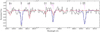 |
Fig. 1 Best fit of the three Zr IV lines seen in the CASPEC spectrum with a resulting abundance of log Zr/H = −5.0. A synthetic spectrum computed without the contribution of Zr is shown as comparison in red. |
Abundance results by number relative to hydrogen (log N(X)/N(H)), by number fraction (log ɛ), and number fraction relative to solar (log ɛ/ɛ⊙).
3.1 Optical spectrum
Although the S/N of the CASPEC spectrum is only moderately high, a fair amount of metallic lines are visible. The vast majority of these lines originates from carbon, nitrogen, and oxygen transitions. The strongest lines were individually fit, and we found C and N to be slightly enriched with respect to the solar values, while O is depleted by a factor of ten. The abundances obtained from the optical lines also reproduce the C, N, and O lines in the UV range well. The only exception is the C III line at 1329.2 Å, which is too strong in the model, although other UV lines of C III are properly reproduced. The Mg abundance derived from the weak Mg II λ4481 line is slightly subsolar. Because no other Mg line is visible and the detected line is weak, we adopt this abundance as an upper limit.
The CASPEC spectrum of Feige 46 also features three relatively strong Zr IV lines. Zirconium lines have so far only been identified in the optical spectra of three other hot subdwarfs, all of which belong to the intermediate helium-rich spectral class (Naslim et al. 2011, 2013; Dorsch et al. 2019). The fit of the three Zr lines resulted in an abundance of log Zr/H = −5.0, which translates into an enrichment of about 20 000 with respect to the solar abundance. The best fit to the Zr lines is presented in Fig. 1. The Zr abundance derived from the optical lines is further supported by the two lines in the GHRS range (Zr IV λλ1441, 1469.5).
The Y III lines (λλ4039.602, 4040.112) are also visible, although the quality of the spectrum in that region is poor. The lines are well reproduced with an abundance of log Y/H = −5.0. Unfortunately, these spectral lines are the only yttrium features identified so far in hot subdwarfs. Oscillator strengths for additional yttrium lines, particularly Y IV, or a higher quality optical spectrum of Feige 46 would be helpful to confirm our abundance value. Nevertheless, the abundances derived for both Zr and Y suggest an enrichment similar to that seen in LS IV − 14°116. A comparison between the full CASPEC spectrum and our final model is shown in Fig. C.1.
3.2 UV spectra
Although the abundances that can be reliably derived with the optical spectrum are limited to a few elements, the UV range covered by the GHRS spectra, and supplemented by the IUE spectrum, allowed us to derive abundances of 11 additional elements. The comparison between the UV spectra and our final model of Feige 46 is shown in Figs. C.2 and C.3, while the values derived for all atomic species are listed in Table 1. Below we summarize the chemical composition obtained from the UV observations.
Iron and nickel show numerous lines over the GHRS ranges, and their abundances were obtained by fitting multiple wavelength ranges that mostly contain lines of iron or nickel. The estimated iron abundance is slightly below the solar value, while the nickel abundance is about ten times solar. With the iron and nickel abundances set to their best-fit values, the same method was applied to derive the abundances of the iron-group elements Cr, Co, and Zn. The Mn lines are all relatively weak and strongly blended in the GHRS range. We derived an upper limit of log Mn/H < −5.7 using several blended lines (e.g., Mn IV λλ1340.66, 1341.93, and 1442.83).
The two Si IV resonance lines indicate an abundance of log Si/H = −5.9 ± 0.1, meaning that this element is depleted in the star. We used the S V λ1501.76 line to derive an upper limit of 1/10 solar for sulfur. We also identified some strong Ti lines, most notably Ti IV λλ1451.74, 1467.34, 1469.19, andTi IIIλ1455.20. Fitting these lines gives an abundance of log Ti/H = −5.69 ± 0.15, which is about 17 times solar.
The GHRS spectra cover several Ga IV lines (Ga IV λλ1338.13, 1347.08, 1351.07, 1395.55, and 1402.61), but also the very strong Ga III λ1495.045 line. We derived an abundance of log Ga/H = −5.2 ± 0.4 from these lines, about 4000 times solar. The Ga III 1507.96 Å line listed in Morton (2003) was excluded from our models because it is not observed at the stated position and was also discrepant in the spectrum of HZ 44 (Dorsch et al. 2019). The strongest Sr line in the GHRS spectra of Feige 46 is by far Sr IV λ1331.13, although several weaker lines are alsovisible (e.g., Sr IVλλ 1394.94, 1492.07). A comparison with synthetic spectra is shown in Fig. 2 and suggests an abundance of log Sr/H = −4.4 ± 0.4, which is more than 4 dex higher than the solar value.
The Ge IV λ1229.84 resonance line is visible in the low S/N IUE spectrum of Feige 46 (see Fig. 3), while the GHRS data cover only the two blended Ge IV lines (λλ 1494.89, 1500.61). From these lines we derived log Ge/H = −5.8 ± 0.6. The Sn IV resonance lines (λλ 1314.54, 1437.53) are outside of the GHRS ranges but are visible in the IUE spectrum (Fig. 3). Based on these features, we estimated an abundance of log Sn/H = −6.0 ± 0.6. We note, however, that the predicted Sn III line at 1251.4 Å does not appear in the observation. This is reminiscent of the problem discussed in Latour et al. (2016). The discrepancy observed by the authors, although in a colder sdB, was similar: the abundance indicated by the fit of the Sn IV lines produced an Sn III line much stronger than observed.
A final element that is interesting in the context of heavy metal enrichment is lead. Unfortunately, the GHRS ranges do not cover strong Pb lines, but the Pb IV line at 1313 Å in the IUE spectrum (Fig. 3) excludes Pb abundances higher than log Pb/H ≲−7.3 (700 times solar). Because the only lead line that we could identify is in the IUE spectrum and not particularly strong (compared to the Sn IV resonance doublet), we prefer to state only an upper limit on the Pb abundance. We note that O’Toole (2004) reported thedetection of Pb in the GHRS observation of Feige 46, although it is not mentioned which lines were detected in that star. Unfortunately, the Pb lines that were investigated by the authors, and that are in the GHRS ranges, have no available oscillator strenghts.
In addition to the elements mentioned above, we also searched for lines of other chemical species that have been observed in hot subdwarfs, for example, P, Al, Ar, and V. No convincing identification or abundances could be determined, although in some cases we tentatively estimated an upper limit. We include a short discussion of these additional elements in Appendix B.
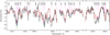 |
Fig. 2 Some of the strongest Sr IV lines in the GHRS spectra compared with synthetic spectra including [Sr/H] = −4.0 (green), −4.4 (blue), and −4.8 (red) and without the contribution of Sr (dashed red). |
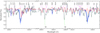 |
Fig. 3 Comparison between the IUE and synthetic spectra in the ranges where Ge, Sn, and Pb lines are seen. The modelspectra shown in blue include the estimated abundances of Ge and Sn (from Table 1); the uncertainty range is indicated by a shaded area. The lower bound of the shaded area for the Pb line represents the upper limit for Pb listed in Table 1 plus its uncertainty (i.e., log Pb/H = −6.7). A synthetic spectrum computed without the contribution of Ge, Sn, and Pb is shown as comparison in red. All spectra are smoothed with a three-pixel box filter for clarity. |
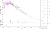 |
Fig. 4 Comparison of the synthetic spectrum (gray line) of Feige 46 with photometric data. The three black data points labeled “box” are binned fluxes from a low-dispersion IUE spectrum. Filter-averaged fluxes are shown as colored data points that were converted from observed magnitudes (the dashed horizontal lines indicate the respective filter widths). The residual panels at the bottom and right-hand side show the differences between synthetic and observed magnitudes and colors, respectively. The following color codes are used to identify the photometric systems: Johnson-Cousins (blue), Strömgren (green), Gaia (cyan), UKIDSS (rose), and 2MASS (red). |
4 Spectral energy distribution and stellar mass
Photometry,which is apparent magnitudes and colors, provides important information to constrain the angular diameter of a star. We used photometric measurements from the ultraviolet to the infrared as listed in Table C.1 to construct the observed spectral energy distribution (SED) of Feige 46. For the theoretical SED, shown in gray in Fig. 4, we used our final synthetic spectrum of the star. Interstellar reddening was also taken into account by multiplying the synthetic flux with a reddening factor 10−0.4A(λ) using the extinction curve of Fitzpatrick (1999) and assuming an extinction parameter RV = A(V)∕E(B–V) = 3.15.
We derived the angular diameter (Θ) and the interstellar reddening E(B–V) by matching the observations with the synthetic SED and color indices obtained from the final model through χ2 minimization (for details see Heber et al. 2018). The residuals of the SED and color fits are shown in Fig. 4 along with the SED, where the y-axis represents the flux density multiplied by the wavelength to the power of three (Fλ λ3). This y-axis quantity reduces the otherwise steep slope of the SED on such a broad wavelength range. The angular diameter and interstellar reddening obtained from the fit are listed in Table 2, as well as additional parameters that can be further derived: radius, mass, and luminosity.
The stellar radius is obtained from the angular diameter and the parallax (ϖ),
 (1)
(1)
The stellar mass is derived from the surface gravity (log g = 5.93 ± 0.10), the angular diameter, and the parallax through
 (2)
(2)
Finally, the effective temperature (Teff = 36 100 ± 500 K) is also used to derive the luminosity from
 (3)
(3)
The stellar mass obtained is somewhat higher than although consistent with the canonical EHB mass for the core-helium flash (0.46 M⊙).
Parallax and parameters derived from the SED fitting.
5 Discussion
The strong enrichment measured for Sr, Y, and Zr readily confirmed our initial suspicion that Feige 46 belongs to the group of iHe subdwarfs that are also enriched in heavy metals. We summarize the chemical composition of Feige 46 in Fig. 5 and include that of LS IV − 14°116 as well as HZ 44, another iHe subdwarf, as a comparison. The abundance pattern of Ge, Sr, Y, and Zr in the two pulsators is strikingly similar: the latter three elements are similarly enhanced by more than 10 000× with respect to the solar abundances. The abundance pattern of C, N, O, Mg, and Si is also alike in both stars. Unfortunately, the limited wavelength range of the optical spectrum of LS IV − 14°116 analyzed by Naslim et al. (2011) did not provide much information on the abundance of elements between sulfur and gallium. We recall here that Feige 46 is about 1000 K hotter than LS IV − 14°116 and more He-enriched by ~0.3 dex. On the other hand, the abundances of HZ 44 show clear differences with respect to the other two stars. Although HZ 44 is also enriched in heavy metals, the abundances of Sr, Y, and Zr are not as high and Pb is the most enriched element in this star. In addition, the abundance pattern of the light elements is different: C and N follow the CNO cycle pattern, with carbon depletion and nitrogen enrichment, and the elements from Ne to Ar are slightly enriched with respect to solar, while they appear to be mostly depleted in the two pulsators. The iron-group elements, however, follow a similar pattern in Feige 46 and HZ 44, and are enriched, except for iron. HZ 44 is hotter (~39 000 K) and more helium rich (log He/H = 0.08) than the two pulsators.
Only a few heavy metal iHe subdwarfs have an extensive abundance portrait, which is partly due to the fact that deriving abundances for most of the iron-group elements requires UV spectroscopy. As seen for Feige 46, UV observations are also valuable to derive abundances of elements such as Ga, Ge, Sr, Sn, and Pb. With incomplete chemical portraits for many of the heavy metal subdwarfs, it is difficult to make proper comparisons. Nevertheless, Feige 46 and LS IV − 14°116 are so far the only iHe-sdOBs with such high overabundances (~3.0−4.5 dex) of Ge, Sr, Y, and Zr. Only one other star currently has a known enrichment of the same order of magnitude in Y and Zr, but its abundance of Ge and Sr is unconstrained (HE 2359-2844, Naslim et al. 2013).
The spectral lines of Feige 46 required an additional broadening that we were able to reproduce by applying a rotational broadening of v sin i = 10 km s−1 to the synthetic spectra. However, this does not necessarily imply that the broadening observed is caused by stellar rotation. On the one hand, the Fourier analysis of the stellar light curve revealed peaks that might be associated with rotational splitting, indicating a rather long rotation period of ~40 days (Latour et al. 2019). On the other hand, Jeffery et al. (2015) showed that the atmospheric motion due to pulsations in LS IV − 14°116 produces radial velocity variations with an amplitude of ≈5 km s−1. It is thus possible that the pulsations in Feige 46 are responsible for the additional broadening because the exposure time of our different spectra are long enough (1500−5400 s) to cover a significant fraction of the pulsation periods (2294−3400 s). Broadening due to pulsations has also been reported in other sdBs (Kuassivi et al. 2005; Telting et al. 2008; Van Grootel et al. 2019). The planned observations of Feige 46 by the Transiting Exoplanet Survey Satellite (Ricker et al. 2014) in sector 22 are expected to provide a longer (27 days) light curve that will allow us to confirm the presence of rotational splitting and provide a better estimate of the rotation period.
An alternative mechanism that could produce line broadening is microturbulent velocity. For instance, in their analysis of LS IV − 14°116, Naslim et al. (2011) adopted a microturbulent velocity of vt = 10 km s−1 based on six optical C III lines. However, Jeffery et al. (2017) found the optical N III lines in [CW83] 0825+15, another iHe subdwarfs with overabundances of Y and Pb, to be rather insensitive to vt and adopted a value of vt = 2 km s−1. To investigate the effect of microturbulence, we computed additional synthetic spectra with vt = 5 km s−1 and no rotational broadening. We compared this spectrum with our current best model (including vt = 2 km s−1) and the spectra of Feige 46 around the Zr IV lines in Fig. 6. While the optical Zr lines are only very weakly affected by the change in microturbulent velocity, the stronger lines in the UV become significantly deeper with increasing microturbulence. While the Zr abundance derived from the optical lines (log Zr/H = −5.0) with rotational broadening reproduces the Zr lines seen in the GHRS spectra well, this is not the case when the microturbulence is increased. Following this comparison, increasing the microturbulent velocity does not appear as a suitable option to reproduce the observed line broadening.
 |
Fig. 5 Comparison between the abundance pattern of Feige 46, LSIV– 14°116 (Naslim et al. 2011) and HZ 44 (Dorsch et al. 2019). Light elements (23 ≤ Z) are marked by green symbols, iron-peak elements (24 ≤ Z ≤ 30) are plotted in purple, and heavier elements (Z ≥ 31) in red. |
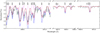 |
Fig. 6 Comparison between the observed spectra and synthetic spectra with vt = 2 km s−1, v sin i = 12 km s−1 (red) and vt = 5 km s−1, v sin i = 0 km s−1 (blue). |
6 Conclusion
We performed an abundance analysis of the pulsating iHe-sdOB star Feige 46 using optical and UV spectroscopic data. This allowed us to derive abundances for 16 metallic elements, including Ge, Sr, Y, Zr, and Sn. Our results not only confirmed that the star belongs to the small class of heavy metal hot subdwarfs, but also showed that Feige 46 and LS IV − 14°116, the only two members of the V366 Aqr pulsating class, have a very similar abundance pattern that is characterized by extreme overabundances of Sr, Y, and Zr (~4.0−4.5 dex). None of the handful of other known heavy metal subdwarfs has so far had abundances that reached the values reported in LS IV − 14°116 for this trio of elements. We might wonder about the fact that the only star in which we found enhancement for these three elements as high as in LS IV − 14°116 also displays the same type of pulsations. This might be related to the pulsating nature of the stars, or to their halo kinematics. With so few abundances and upper limit constraints in other stars, we unfortunately cannot draw any conclusions yet. The only two stars with a complete set of values and upper limits for Sr, Y, Zr, as well as Ge and Pb are the two hotter and more He-rich stars (including HZ 44) that were analyzed by Dorsch et al. (2019). In these two stars, the enrichment in Ge, Sr, Y, and Zr is not as high as in the pulsators, although their Pb abundance is higher than in Feige 46. With radiative levitation likely playing a role in supporting such high abundances of these elements in the line-forming region, the effective temperature of the stars would influence their photospheric abundances. The temperature region at which Feige 46 and LS IV − 14°116 are found (~35 500–37 000 K) might well be ideal for the radiative support of Sr, Y, and Zr. On the other hand, it is not clear whether radiative levitation can build up such high overabundances from an initial solar-like amount, and additional production of heavy elements, for example, during the recent evolution of the star, might be required.
Acknowledgements
We thank Andreas Irrgang and Simon Kreuzer for the development of the SED fitting tool. M.L. acknowledges funding from the Deutsche Forschungsgemeinschaft (grant DR 281/35-1). This research has made use of NASA’s Astrophysics Data System. Based on observations made with the NASA/ESA Hubble Space Telescope, obtained from the MAST archive (prop. ID GO5319, P.I: Heber) at the Space Telescope Science Institute. STScI is operated by the Association of Universities for Research in Astronomy, Inc. under NASA contract NAS 5-26 555.
Appendix A Partition functions
For chemicalelements with atomic number Z ≤ 30, the necessary data to include a line in LTE are already implemented in Synspec 51 for all relevant ionization stages. For heavier elements, however, only the stages I-II-III are implemented. In sdOB stars, many elements are more highly ionized; the dominant stages are IV-V. Thus additional atomic data had to be supplemented to allow the inclusion of lines from heavy elements such as Ge, As, Zr, and Pb. Table A.1 lists the number of levels considered for each additional ion and their ionization energy (χI). We used thenon-standard PFSPEC subroutine in SYNSPEC to compute partition functions for these ions as it was already implemented and used for C VI, N VI-VII, and O VI-VIII. Although the subroutine includes the possibility to account for level dissolution and electron shielding, we used the Boltzmann equation to compute the partition function (U) of the additional ions,
![Mathematical equation: \begin{equation*} \begin{split} &U_i = g_i\cdot \exp (-E_i/k_{\textrm{B}}T)\\%[2pt] &U = \sum _i U_i.\\[-7pt] \end{split} \end{equation*}](/articles/aa/full_html/2019/09/aa36247-19/aa36247-19-eq4.png)
Number of new levels per ion added to SYNSPEC and the corresponding ionization potentials.
For each level i, gi is the statistical weight, Ei is the energy of the level, and kB is the Boltzmann constant.
Appendix B Additional chemical elements
We also searched for lines of Al, P, Ar, Ca, Sc, V, Kr, Nb, Mo, In, Te, and Xe and describe our results below.
Two Al III lines are predicted in the GHRS range, Al III 1379.67 Å matches an unidentified line with log Al/H = −5.6, but the Al III line at 1348.13 Å is too strong at this abundance and is more consistent with log Al/H = −6.2.
Phosphorus abundances higher than log P/H = −5.4 are excluded by several lines (e.g., P III λλ 1334.81, 1344.33, 1344.85, P IV 1467.43, 1484.51, and 1487.79). The two P III lines at 1334.81 and 1344.33 Å also exclude abundances higher than log P/H = −6.0.
No argon lines could be clearly identified in the GHRS range, but abundances higher than log Ar/H = −3.2 can be excluded. The Ca III lines λλ1461.89, 1463.34, 1484.87, and 1496.88 exclude abundances higher than log Ca/H = −4.0.
Vanadium at an abundance of V/H = −6.0 improves the GHRS fit in some blended regions, and the V IV lines at 1355.13 and 1403.61 Å would match otherwise unidentified lines. This is not reliable enough for an abundance measurement, but an upper limit of V/H = −5.4 can be estimated because many V lines are too strong at this abundance.
We searched for niobium using Nb IV oscillator strengths provided by Tauheed & Reader (2005). Several unidentified weak lines in the GHRS spectrum (e.g., Nb IV λλ1445.74, 1473.44, and 1508.72) can be reproduced with an abundance of log Nb/H = −5.9. Other Nb IV lines such as λλ1330.60, 1447.49, 1487.26, and 1517.46 favor a lower abundance of log Nb/H = −6.3.
A molybdenum abundance of log Mo/H = −6.2 improves the overall match between the observations and our best model. The Mo abundance could be higher because several lines of that element fit with abundances up to log Mo/H = −5.6 (e.g., Mo IV 1455.86, 1456.32, and 1458.04 Å). However, a few Mo lines are too strong when log Mo/H = −5.6 is adopted (e.g., Mo IV 1351.27, 1412.43, and 1440.87 Å).
Three noteworthy In III lines lie in the GHRS range: λλ1403.08, 1487.67, and 1494.11. The 1403.08 Å line fits a strong, unidentified line with log In/H = −5.4 that is excluded by the other two lines. This line is also blended with a weak Ni III line that could be underestimated in the model. On the other hand, the In III 1487.67 would exclude abundances higher than log In/H = −6.5.
Finally, predicted scandium, krypton, tellurium, and xenon lines are all very weak, and no meaningful upper limit could be estimated.
Appendix C Additional material
C.1 Full spectral comparisons
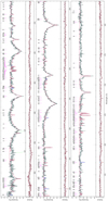 |
Fig. C.1 CASPEC spectrum of Feige 46 (gray) and the final model with vrot sin i = 10 km s−1 in red; the model in blue also includes lines from heavy elements (Z > 30). Mismatches of broad lines are due to shortcomings of the normalization procedure. This does not compromise the measurement of sharp metal lines, however. |
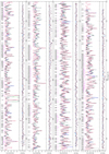 |
Fig. C.2 GHRS spectrum of Feige 46 (gray) and the final model with vrot sin i = 10 km s−1 in red; the model in blue also includes lines from heavy elements (Z > 30). |
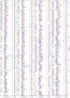 |
Fig. C.3 Part of the IUE spectrum of Feige 46 (gray) and the final model with vrot sin i = 10 km s−1 in red; the model in blue also includes lines from heavy elements (Z > 30). All spectra are smoothed with a three-pixel box filter, and the regions with bad data points in the IUE spectrum are not drawn. |
C.2 Photometric data
Photometric data used for the SED-fit of Feige 46.
References
- Battich, T., Bertolami, M. M. M., Córsico, A. H., & Althaus, L. G. 2018, A&A, 614, A136 [NASA ADS] [CrossRef] [EDP Sciences] [Google Scholar]
- Bauer, F., & Husfeld, D. 1995, A&A, 300, 481 [NASA ADS] [Google Scholar]
- Blanchette, J.-P., Chayer, P., Wesemael, F., et al. 2008, ApJ, 678, 1329 [NASA ADS] [CrossRef] [Google Scholar]
- Brown, T. M., Sweigart, A. V., Lanz, T., Landsman, W. B., & Hubeny, I. 2001, ApJ, 562, 368 [NASA ADS] [CrossRef] [Google Scholar]
- Chambers, K. C., Magnier, E. A., Metcalfe, N., et al. 2016, ArXiv e-prints [arXiv:1612.05560] [Google Scholar]
- Chayer, P., Fontaine, M., Fontaine, G., Wesemael, F., & Dupuis, J. 2006, Balt. Astron., 15, 131 [NASA ADS] [Google Scholar]
- Dorman, B., Rood, R. T., & O’Connell, R. W. 1993, ApJ, 419, 596 [CrossRef] [Google Scholar]
- Dorsch, M., Latour, M., & Heber, U. 2019, A&A, in press, https://doi.org/10.1051/0004-6361/201935724 [Google Scholar]
- Drilling, J. S., & Heber, U. 1987, in Second Conference on Faint Blue Stars, IAU Colloq. 95, eds. A. G. D. Philip, D. S. Hayes, & J. W. Liebert (Schenectady, N.Y.: L. Davis Press), 603 [Google Scholar]
- Fitzpatrick, E. L. 1999, PASP, 111, 63 [NASA ADS] [CrossRef] [Google Scholar]
- Gaia Collaboration 2018, VizieR Online Data Catalog: I/345 [Google Scholar]
- Geier, S., Østensen, R. H., Nemeth, P., et al. 2017, Open Astron., 26, 164 [NASA ADS] [CrossRef] [Google Scholar]
- Graham, J. A. 1970, PASP, 82, 1305 [NASA ADS] [CrossRef] [Google Scholar]
- Heber, U. 2016, PASP, 128, 082001 [NASA ADS] [CrossRef] [Google Scholar]
- Heber, U., Irrgang, A., & Schaffenroth, J. 2018, Open Astron., 27, 35 [Google Scholar]
- Hirsch, H. A. 2009, PhD Thesis, Friedrich-Alexander University Erlangen-Nürnberg, Germany [Google Scholar]
- Hu, H., Tout, C. A., Glebbeek, E., & Dupret, M.-A. 2011, MNRAS, 418, 195 [NASA ADS] [CrossRef] [Google Scholar]
- Hubeny, I. 1988, Comput. Phys. Commun., 52, 103 [NASA ADS] [CrossRef] [Google Scholar]
- Hubeny, I., & Lanz, T. 2011, Astrophysics Source Code Library [record ascl:1109.021] [Google Scholar]
- Jeffery, C. S., Ahmad, A., Naslim, N., & Kerzendorf, W. 2015, MNRAS, 446, 1889 [NASA ADS] [CrossRef] [Google Scholar]
- Jeffery, C. S., Baran, A. S., Behara, N. T., et al. 2017, MNRAS, 465, 3101 [NASA ADS] [CrossRef] [Google Scholar]
- Kuassivi, B. A., & Ferlet, R. 2005, A&A, 442, 1015 [NASA ADS] [CrossRef] [EDP Sciences] [Google Scholar]
- Lanz, T., & Hubeny, I. 2003, ApJS, 146, 417 [NASA ADS] [CrossRef] [Google Scholar]
- Latour, M., Fontaine, G., Chayer, P., & Brassard, P. 2013, ApJ, 773, 84 [NASA ADS] [CrossRef] [Google Scholar]
- Latour, M., Heber, U., Irrgang, A., et al. 2016, A&A, 585, A115 [NASA ADS] [CrossRef] [EDP Sciences] [Google Scholar]
- Latour, M., Green, E. M., & Fontaine, G. 2019, A&A, 623, L12 [NASA ADS] [CrossRef] [EDP Sciences] [Google Scholar]
- Lawrence, A., Warren, S. J., Almaini, O., et al. 2013, VizieR Online Data Catalog, II/319 [Google Scholar]
- Mermilliod, J. C. 2006, VizieR Online Data Catalog, II/168 [Google Scholar]
- Michaud, G., Richer, J., & Richard, O. 2011, A&A, 529, A60 [NASA ADS] [CrossRef] [EDP Sciences] [Google Scholar]
- Miller Bertolami, M. M., Córsico, A. H., & Althaus, L. G. 2011, ApJ, 741, L3 [NASA ADS] [CrossRef] [Google Scholar]
- Morton, D. C. 2000, ApJS, 130, 403 [NASA ADS] [CrossRef] [MathSciNet] [Google Scholar]
- Morton, D. C. 2003, ApJS, 149, 205 [NASA ADS] [CrossRef] [MathSciNet] [Google Scholar]
- Naslim, N., Jeffery, C. S., Behara, N. T., & Hibbert, A. 2011, MNRAS, 412, 363 [NASA ADS] [CrossRef] [Google Scholar]
- Naslim, N., Jeffery, C. S., Hibbert, A., & Behara, N. T. 2013, MNRAS, 434, 1920 [NASA ADS] [CrossRef] [Google Scholar]
- O’Toole, S. J. 2004, A&A, 423, L25 [NASA ADS] [CrossRef] [EDP Sciences] [Google Scholar]
- O’Toole, S. J., & Heber, U. 2006, A&A, 452, 579 [NASA ADS] [CrossRef] [EDP Sciences] [Google Scholar]
- Randall, S. K., Bagnulo, S., Ziegerer, E., Geier, S., & Fontaine, G. 2015, A&A, 576, A65 [NASA ADS] [CrossRef] [EDP Sciences] [Google Scholar]
- Rauch, T., Quinet, P., Hoyer, D., et al. 2015, Tuebingen Oscillator Strengths Service Form Interface, VO resource provided by the GAVO Data Center [Google Scholar]
- Ricker, G. R., Winn, J. N., Vanderspek, R., et al. 2014, Proc. SPIE, 9143, 914320 [Google Scholar]
- Saio, H., & Jeffery, C. S. 2019, MNRAS, 482, 758 [NASA ADS] [CrossRef] [Google Scholar]
- Stroeer, A., Heber, U., Lisker, T., et al. 2007, A&A, 462, 269 [NASA ADS] [CrossRef] [EDP Sciences] [Google Scholar]
- Tauheed, A., & Reader, J. 2005, Phys. Scr., 72, 158 [NASA ADS] [CrossRef] [Google Scholar]
- Telting, J. H., Geier, S., Østensen, R. H., et al. 2008, A&A, 492, 815 [NASA ADS] [CrossRef] [EDP Sciences] [Google Scholar]
- Unglaub, K. 2008, A&A, 486, 923 [NASA ADS] [CrossRef] [EDP Sciences] [Google Scholar]
- Van Grootel, V., Randall, S. K., Latour, M., et al. 2019, ArXiv e-prints [arXiv:1905.00654] [Google Scholar]
- van Hoof, P. A. M. 2018, Galaxies, 6, 63 [NASA ADS] [CrossRef] [Google Scholar]
- Wamsteker, W., Skillen, I., Ponz, J., et al. 2000, Astrophys. Space Sci., 273, 155 [NASA ADS] [CrossRef] [Google Scholar]
- Werner, K., Dreizler, S., & Rauch, T. 2012, Astrophysics Source Code Library [record ascl:1212.015] [Google Scholar]
- Williams, T., McGraw, J. T., Mason, P. A., & Grashuis, R. 2001, PASP, 113, 944 [NASA ADS] [CrossRef] [Google Scholar]
- Zhang, X., & Jeffery, C. S. 2012, MNRAS, 419, 452 [NASA ADS] [CrossRef] [Google Scholar]
All Tables
Abundance results by number relative to hydrogen (log N(X)/N(H)), by number fraction (log ɛ), and number fraction relative to solar (log ɛ/ɛ⊙).
Number of new levels per ion added to SYNSPEC and the corresponding ionization potentials.
All Figures
|
Fig. 1 Best fit of the three Zr IV lines seen in the CASPEC spectrum with a resulting abundance of log Zr/H = −5.0. A synthetic spectrum computed without the contribution of Zr is shown as comparison in red. |
| In the text | |
|
Fig. 2 Some of the strongest Sr IV lines in the GHRS spectra compared with synthetic spectra including [Sr/H] = −4.0 (green), −4.4 (blue), and −4.8 (red) and without the contribution of Sr (dashed red). |
| In the text | |
|
Fig. 3 Comparison between the IUE and synthetic spectra in the ranges where Ge, Sn, and Pb lines are seen. The modelspectra shown in blue include the estimated abundances of Ge and Sn (from Table 1); the uncertainty range is indicated by a shaded area. The lower bound of the shaded area for the Pb line represents the upper limit for Pb listed in Table 1 plus its uncertainty (i.e., log Pb/H = −6.7). A synthetic spectrum computed without the contribution of Ge, Sn, and Pb is shown as comparison in red. All spectra are smoothed with a three-pixel box filter for clarity. |
| In the text | |
|
Fig. 4 Comparison of the synthetic spectrum (gray line) of Feige 46 with photometric data. The three black data points labeled “box” are binned fluxes from a low-dispersion IUE spectrum. Filter-averaged fluxes are shown as colored data points that were converted from observed magnitudes (the dashed horizontal lines indicate the respective filter widths). The residual panels at the bottom and right-hand side show the differences between synthetic and observed magnitudes and colors, respectively. The following color codes are used to identify the photometric systems: Johnson-Cousins (blue), Strömgren (green), Gaia (cyan), UKIDSS (rose), and 2MASS (red). |
| In the text | |
|
Fig. 5 Comparison between the abundance pattern of Feige 46, LSIV– 14°116 (Naslim et al. 2011) and HZ 44 (Dorsch et al. 2019). Light elements (23 ≤ Z) are marked by green symbols, iron-peak elements (24 ≤ Z ≤ 30) are plotted in purple, and heavier elements (Z ≥ 31) in red. |
| In the text | |
|
Fig. 6 Comparison between the observed spectra and synthetic spectra with vt = 2 km s−1, v sin i = 12 km s−1 (red) and vt = 5 km s−1, v sin i = 0 km s−1 (blue). |
| In the text | |
|
Fig. C.1 CASPEC spectrum of Feige 46 (gray) and the final model with vrot sin i = 10 km s−1 in red; the model in blue also includes lines from heavy elements (Z > 30). Mismatches of broad lines are due to shortcomings of the normalization procedure. This does not compromise the measurement of sharp metal lines, however. |
| In the text | |
|
Fig. C.2 GHRS spectrum of Feige 46 (gray) and the final model with vrot sin i = 10 km s−1 in red; the model in blue also includes lines from heavy elements (Z > 30). |
| In the text | |
|
Fig. C.3 Part of the IUE spectrum of Feige 46 (gray) and the final model with vrot sin i = 10 km s−1 in red; the model in blue also includes lines from heavy elements (Z > 30). All spectra are smoothed with a three-pixel box filter, and the regions with bad data points in the IUE spectrum are not drawn. |
| In the text | |
Current usage metrics show cumulative count of Article Views (full-text article views including HTML views, PDF and ePub downloads, according to the available data) and Abstracts Views on Vision4Press platform.
Data correspond to usage on the plateform after 2015. The current usage metrics is available 48-96 hours after online publication and is updated daily on week days.
Initial download of the metrics may take a while.