| Issue |
A&A
Volume 627, July 2019
|
|
|---|---|---|
| Article Number | A93 | |
| Number of page(s) | 8 | |
| Section | Extragalactic astronomy | |
| DOI | https://doi.org/10.1051/0004-6361/201935827 | |
| Published online | 04 July 2019 | |
Ultraviolet photo-ionisation in far-infrared selected sources
1
School of Chemical and Physical Sciences, Victoria University of Wellington, PO Box 600 Wellington 6140, New Zealand
e-mail: Stephen.Curran@vuw.ac.nz
2
International Centre for Radio Astronomy Research (ICRAR), Curtin University, Bentley, WA 6102, Australia
Received:
3
May
2019
Accepted:
31
May
2019
It has been reported that there is a deficit of stellar heated dust, as evident from the lack of far-infrared (FIR) emission, in sources within the Herschel-SPIRE sample with X-ray luminosities exceeding a critical value of LX ∼ 1037 W. Such a scenario would be consistent with the suppression of star formation by the AGN, required by current theoretical models. Since absorption of the 21 cm transition of neutral hydrogen (H I), which traces the star-forming reservoir, also exhibits a critical value in the ultraviolet band (above ionising photon rates of Q ≈ 3 × 1056 s−1), we test the SPIRE sample for the incidence of the detection of 250 μm emission with Q. The highest value at which FIR emission is detected above the SPIRE confusion limit is Q = 8.9 × 1057 s−1, which is ≈30 times that for the H I, with no critical value apparent. Since complete ionisation of the neutral atomic gas is expected at Q ≳ 3 × 1056 s−1, this may suggest that much of the FIR must arise from heating of the dust by the AGN. However, integrating the ionising photon rate of each star over the initial mass function, we cannot rule out that the high observed ionising photon rates are due to a population of hot, massive stars.
Key words: galaxies: active / ultraviolet: galaxies / infrared: galaxies / X-rays: galaxies / galaxies: ISM / submillimeter: galaxies
© ESO 2019
1. Introduction
Feedback between active galactic nuclei (AGN) and their host galaxies is complex, with the central engine ionising the very material which feeds it (e.g. Di Matteo et al. 2005; Fabian 2012). The ionisation can arise from powerful outflows into the surrounding neutral medium (jet/radio-mode; e.g. Cano-Díaz et al. 2012; Farrah et al. 2012), as well as by ultraviolet (Silk & Rees 1998) and X-ray (Fabian 1999) radiation emanating from the accretion disc surrounding the supermassive black hole (radiative/quasar-mode, Hardcastle et al. 2007; Heckman & Best 2014). Both mechanisms suppress star formation through ionisation and heating of the neutral gas, this suppression being required by current theoretical models to reproduce the observed properties of active galaxies (e.g. Croton et al. 2006). Observational evidence of this has recently been claimed, where powerful AGN, as evident through their X-ray luminosity, lack λ = 250 μm far-infrared (FIR) emission over the redshift range 1 < z < 3. In the rest frame this corresponds to wavelengths of 63 − 125 μm, which trace the dust heated by stars (e.g. Dale & Helou 2002), and so the absence of FIR emission is interpreted as the suppression of star formation in the X-ray luminous sources (Page et al. 2012).
Powerful AGN are also extremely bright in the UV, which is redshifted into the optical band at z ≳ 3, allowing quasi-stellar objects (QSOs) to be visible to ground-based telescopes over much of the observable Universe. Observational evidence of high UV luminosities rendering the star-forming material undetectable in the hosts of radio-loud QSOs (quasars) was suggested by the exclusive non-detection of the 21 cm transition of neutral hydrogen (H I) above a critical UV luminosity of LUV ∼ 1023 W Hz−1 (Curran et al. 2008). H I 21 cm absorption traces the cool, star forming, component of the gas and a subsequent model of a quasar placed within an exponential gas disc found that this luminosity, which corresponds to Q ∼ 3 × 1056 ionising (λ ≤ 912 Å) photons s−1, is just sufficient to ionise all of the neutral gas in the Milky Way (Curran & Whiting 2012). Given that this is a large spiral galaxy, complete ionisation of the neutral gas would explain why H I has never yet been detected in sources with these UV luminosities (Curran et al. 2008, 2011, 2013a,b, 2016, 2017a,b, 2019; Allison et al. 2012; Grasha & Darling 2011; Geréb et al. 2015; Aditya et al. 2016, 2017; Aditya & Kanekar 2018; Curran & Duchesne 2018; Grasha et al. 2019). Since H I 21 cm absorption traces the reservoir for star formation, we may also expect the 250 μm emission to be absent in the sources above the critical UV ionising photon rate, a possibility we investigate here.
2. Analysis
2.1. Source matching
The Herschel Multi-tiered Extragalactic Survey (HerMES, Oliver et al. 2012), utilised by Page et al. (2012), covers a ∼340 deg2 field, operating at wavelengths of λ = 250, 350, and 500 μm (Spectral and Photometric Imaging Receiver, SPIRE) and 100 and 160 μm (Photodetector Array Camera and Spectrometer, PACS). We constructed a subset of extragalactic sources within the SPIRE dataset using the STARFINDER source-finder software (Diolaiti et al. 2000), with cross-identification being performed between the single-band catalogues (Roseboom et al. 2010), resulting in a merged catalogue of 340 968 sources. We then searched the NASA/IPAC Extragalactic Database (NED) for sources within 6 arcsec of the SPIRE positions (as per Page et al. 2012, see Appendix A), which were cross-matched according to the minimum separation between sources, while ensuring no duplicate matches. After filtering out SPIRE sources without a counterpart nor a redshift, there were 62 073 sources remaining. Of these, 14 457 have spectroscopic redshifts (Fig. 1).
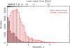 |
Fig. 1. Distribution of the spectroscopic (filled histogram) and the photometric redshifts (unfilled) for the 62 073 matched SPIRE sources. |
2.2. Photometry fitting
2.2.1. Ultraviolet
In order to obtain the UV luminosities, we queried NED, the Wide-Field Infrared Survey Explorer (WISE, Wright et al. 2010), the Two Micron All Sky Survey (2MASS, Skrutskie et al. 2006) and the Galaxy Evolution Explorer (GALEX data release GR6/7)1 databases. Each flux density measurement, Sν, was corrected for Galactic extinction (Schlegel et al. 1998) before being converted to a specific luminosity at the source-frame frequency via  , where DL is the luminosity distance to the source.
The ionising photon rate is defined as  (Osterbrock 1989), where ν0 = 3.29 × 10¹⁵ Hz for the ionisation of neutral hydrogen. For the fitting, we require at least three ν ≳ 1015 Hz photometry points to which we fit a power law, giving log10 Lν = α log10 ν + 𝒞 ⇒ Lν = 10𝒞να, where α is the spectral index and 𝒞 the intercept. This gives the ionising photon rate as
![$$ Q = \frac{10^\mathcal{C}}{h}\int ^{\infty }_{\nu _0}\nu ^{\alpha -1}\,\mathrm{d}{\nu } = \frac{10^\mathcal{C}}{\alpha h}\Bigg [\nu ^{\alpha }\Bigg ]^{\infty }_{\nu _0} = \frac{-10^\mathcal{C}}{\alpha h}\nu _0^{\alpha }, $$](/articles/aa/full_html/2019/07/aa35827-19/aa35827-19-eq3.gif)
where α < 0.
2.2.2. Far-infrared
Since we were also interested in the effect of the UV continuum on the dust temperature, we added the photometric data of the three SPIRE bands to that above, where we only included the data detected at Sν > 3σconf, where σconf = 6 mJy is the SPIRE confusion limit (Nguyen et al. 2010; Smith et al. 2012). For Tdust ≲ hν/k (Younger et al. 2009), where h is the Planck constant and k the Boltzmann constant, we fitted a modified blackbody (Fig. 2) spectrum of the form
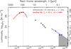 |
Fig. 2. Example of the FIR and UV photometry fits. The vertical line shows the observed-frame 250 μm frequency and the horizontal line the SPIRE confusion limit of 3σconf = 18 mJy. The shaded region shows the λ ≤ 912 Å band over which the ionising photon rate is derived. |
where β is the spectral emissivity index (e.g. Casey 2012).
For this, we used a non-linear least-squares fitting of β and Tdust simultaneously, giving the distribution shown in Fig. 3. This yields a mean dust temperature of ⟨Tdust⟩ = 31 K and a mean spectral emissivity index of ⟨β⟩ = 0.99. This is considerably lower than the canonical β = 1.5 (Blain et al. 2003; Younger et al. 2009 and references therein), although this was used as the initial estimate. Forcing β = 1.5 could not satisfactorily fit the data, although we do note that β ≈ 1.0 may not be unexpected (Hildebrand 1983).
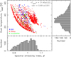 |
Fig. 3. Distribution of spectral emissivity index and dust temperature, where Tdust ≤ 1.2 × 10¹²(z + 1)h/k, giving a sample of n = 2013. The shapes represent the NED classification: stars for QSOs, circles for galaxies, and squares for unclassified. |
3. Effects of the ultraviolet continuum
3.1. Critical ionising photon rate
As stated in the introduction, our main motivation was to test whether the critical ionising photon rate found for H I 21 cm absorption also applied to FIR emission, where an apparent critical X-ray luminosity may suggest the suppression of star formation. The highest ionising photon rate at which 21 cm absorption has been detected is Q = 2.5 × 1056 s−1, above which there are 87 non-detections, which is significant at 5.66σ (Curran et al. 2019). Since 21 cm absorption traces the cool, neutral gas that fuels the star formation, we may therefore expect a similar critical rate if the FIR emission is dominated primarily by stellar activity.
Of the sample, there is sufficient UV photometry for 3315 sources, of which 1347 are considered 250 μm detections (where S250 μm > 18 mJy, Sect. 2.2.2), giving a detection rate of 40.6%. As Fig. 4 shows, unlike for 21 cm absorption, the detections and non-detections share the same range of ionising photon rates, with 250 μm emission being detected up to Q = 8.9 × 1057 s−1. This is considerably higher than that observed for H I 21 cm absorption and the model prediction that all of the neutral gas in a large galaxy is ionised at Q ≳ 3 × 1056 s−1 (Curran & Whiting 2012). Thus, unlike the X-ray emission (Page et al. 2012, but see Appendix A), we see no distinction between the distribution of FIR detections and non-detections at high ionising photon rates.
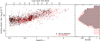 |
Fig. 4. Ionising (λ ≤ 912 Å) photon rate vs. redshift for the sources with spectroscopic redshifts. The filled symbols and histogram represent the FIR detections, unfilled for the non-detections. As in Fig. 3, the shapes represent the NED classification: stars for QSOs, circles for galaxies, and squares for unclassified. |
3.2. Dust heating
Interstellar dust has an absorption cross-section that peaks at ultraviolet wavelengths, thus making the re-emitted FIR radiation a sensitive tracer of dust heating. From the modified blackbody fits to the FIR photometry, we can also investigate heating of the dust by the ultraviolet emission. Of the 250 μm detections, there are 404 sources to which we could fit a modified blackbody and which have sufficient UV photometry (e.g. Fig. 2). These exhibit a strong correlation between the dust temperature and the ionising photon rate (Fig. 5), with a generalised non-parametric Kendall-tau test giving a probability of P(τ) = 5.28 × 10⁻¹² for the Tdust − Q correlation arising by chance, which is significant at S(τ) = 6.90σ assuming Gaussian statistics. However, due to the flux limitation introduced by the SPIRE confusion limit, there will be a bias towards the most FIR luminous, and thus most UV luminous, sources with increasing redshift. Given that for a modified blackbody, the temperature and intensity are not independent (Sect. 2.2.2), this will also lead to an apparent increase in the dust temperature.
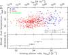 |
Fig. 5. Dust temperature vs. ionising photon rate. Bottom panel: data are shown in equally sized bins. The horizontal bars show the range of points in the bin and the vertical error bars the 1σ uncertainty in the mean value. |
In order to correct for this, we obtained the integrated intensity over 40–1000 μm (Yang et al. 2007, cf. Fig. 2) from
from which a specific intensity (I250 μm) is compared to the corresponding specific luminosity (L250 μm, e.g. Fig. 2) in order to provide the scaling to LFIR (Fig. 6). From this we see that many of the luminosities are in excess of LFIR ≳ 1012 L⊙, qualifying the sources as Ultra-Luminous Infrared Galaxies (ULIRGs). Normalising the ionising photon rate by the FIR luminosity (Fig. 7), the correlation disappears. This and Fig. 6 therefore indicate that the increase in dust temperature with redshift2 is due to the flux limitation introducing a bias towards the most FIR (and UV) luminous sources.
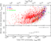 |
Fig. 6. Dust temperature vs. total FIR luminosity. The dashed curve shows the fit for the SPIRE-mm sources (Roseboom et al. 2012). |
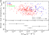 |
Fig. 7. Dust temperature vs. the ionising photon rate normalised by the total FIR luminosity. |
3.3. Stellar versus AGN activity
The FIR emission is believed to be dominated by stellar heating (Rieke & Lebofsky 1979 and references therein), whereas the mid-infrared (MIR, λ = 24 μm) emission can arise in photon dominated or HII regions (e.g. Galliano et al. 2018), and from AGN heated dust in the circumnuclear torus (Hatziminaoglou et al. 2010)3. However, the absence of the same critical ionising photon rate, which completely ionises the neutral atomic gas, and thus suppresses the star formation, at Q ≳ 3 × 1056 s−1 (Curran & Whiting 2012), may suggest that much of the FIR emission also arises from dust heated by the AGN (e.g. de Grijp et al. 1985; Curran et al. 2001; Nardini et al. 2010).
For a blackbody with T = 5770 K and a radius of R⊙ = 696 × 108 m, the ionising photon rate of the Sun is Q⊙ = 7.9 × 1035 s−1. Thus, UV luminosities corresponding to Q ≳ 1057 s−1 (Fig. 4) would require ≳1021 solar mass stars and so, while an older (lower mass) population of stars could contribute significantly to the FIR luminosity (Calzetti et al. 2010; Groves et al. 2012; Li et al. 2013), they cannot account for the UV luminosity. In order to explore the stellar masses required, the ionising photon rate of a star is obtained from the integrated intensity, Iν, via
ν0 = 3.29 × 10¹⁵ Hz corresponds to λ = 912 Å, where the hydrogen is ionised, and T⋆ is the surface temperature of the star. To obtain the luminosity we require a value for the surface area of the star ( ), which we estimate from the comparison of the bolometric intensity,
  , with the bolometric luminosity obtained from the main sequence using log10L⋆ = 6.50log10T⋆ − 24.37. Examples of the derived properties are given in Table 1.
Estimated properties of stars of various temperatures.
In order to obtain the total ionising luminosity, we integrate both the initial mass function (IMF or ξ) and Q⋆ over the whole mass range, which we normalise to the approximate stellar mass of the Milky Way (Fig. 8). The total stellar mass is given by  and it is dominated by the low mass stars, whereas the total ionising photon rate is dominated by the massive stars (see Table 1). If we truncate the IMF at M⋆ = 25 M⊙ (T⋆ ≈ 30 000 K, tMS ≈ 3 × 10⁶ yr) for the maximum possible mass, we obtain Qtotal = 3 × 1056 s−1, whereas setting this to M⋆ = 100 M⊙ (T⋆ ≈ 65 000 K, tMS ≈ 1 × 10⁵ yr) gives Qtotal = 7 × 1057 s−1.
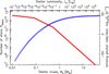 |
Fig. 8. Frequency of various stellar masses obtained from the initial mass function, ξ = ξ0Mα, normalised to give a total stellar mass of Mtotal = 4 × 10¹¹ M⊙, α = −0.3 for 0.01 < M⊙ < 0.08, α = −1.3 for 0.08 < M⊙ < 0.5, and α = −2.35 for M⊙ > 0.5 (Salpeter 1955; Kroupa 2001). The curve (right-hand scale) shows the approximate ionising photon rate per star. |
Thus, the total ionising photon rate from the stellar population within the source is very much dependent upon the upper end of the stellar mass distribution. Assuming no significant AGN contribution, the highest FIR luminosities of the sample indicate star formation rates of ∼104 M⊙ yr−1 (e.g. Kennicutt 1998), which we can use to constrain the upper mass end. In this instance, integrating over all star formation rates4, a total of SFRtotal = 1 × 10⁴ M⊙ yr−1 is reached for a maximum stellar mass of M⋆ ≈ 40 M⊙, which gives Qtotal = 9 × 1056 s−1. However, even at relatively large look-back times, e.g. ∼10 Gyr (z ∼ 2), this implies a total stellar mass of ∼1013 M⊙, for a constant star formation rate over these first ∼3 Gyr. In addition to the total stellar mass, a steeper IMF would affect the stellar contribution to Qtotal, for instance, α = −2.65 for 1 < M⊙ < 10 stars (Bastian et al. 2010), α = −5 for 25 < M⊙ < 120 stars in the Magellanic Clouds (Massey 2002), or α = −2.45 to − 2.85 in external galaxies (Úbeda et al. 2007; Bruzzese et al. 2015; Weisz et al. 2015). We therefore show the total ionising photon for a range of total masses and IMF indices in Table 2.
Total ionising photon rates, Qtotal, for various stellar mass distributions.
Since the total stellar mass is dominated by the more numerous, least massive, cooler stars, ionising photon rates above the critical 21 cm value favour Mtotal ≲ 4 × 10¹¹ M⊙, although it should be borne in mind that SFRtotal = 1 × 10⁴ M⊙ yr−1 is most likely an upper limit, due to an AGN contribution to the FIR luminosity (Morić et al. 2010; Nardini et al. 2010). For example, for a 50% contribution, the critical ionising photon rate is reached by just two of the canonical Galactic models (Mtotal = 4 × 10¹¹ M⊙, Table 3). This still begs the question of how the continual star formation is fuelled, although the stellar contribution to Qtotal will decrease further with an increasing AGN contribution. Furthermore, we have not accounted for shielding by dust nor how much this attenuates the observed UV flux. Also, while the critical Qtotal = 3 × 1056 s−1 is sufficient to ionise all of the neutral atomic gas in the Milky Way (where n ≲ 10 cm−3, Kalberla & Kerp 2009), since Q ∝ n2 (Osterbrock 1989), denser gas (e.g. in molecular clouds where n ≳ 103 cm−3) requires much higher ionising photon rates (Roos et al. 2015). Simulations of a stellar population distributed within a galactic disc would be required in order to determine whether a distribution of UV luminous point sources would result in a Strömgren sphere of infinite radius, as is the case for a single centrally located Q ≳ 1056 s−1 ionising source (Curran & Whiting 2012).
Lastly, as Fig. 6 shows, many of the highest FIR luminous sources are classified as QSOs, and so are known to host a powerful AGN. Although they form only a small fraction (5%) of the sources for which the FIR luminosity can be derived (Fig. 9), we see that the mean luminosity for the QSOs is an order of magnitude higher than for the galaxies (as is also the case for the UV, Fig. 5), lending support to the argument of an AGN contribution to the FIR emission in the most luminous sources. There does remain, however, a number of galaxies with these same luminosities.
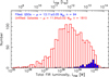 |
Fig. 9. Far-IR luminosity distribution of the known QSOs and galaxies of the sample. |
4. Conclusions
For the past decade evidence has been building of a critical photo-ionisation rate in the ultraviolet band, above which all of the gas in the host galaxy is ionised. All of the observational evidence comes from searches of H I 21 cm absorption in redshifted radio sources, which has never been detected above rates of Q = 2.5 × 1056 s−1 (LUV ≳ 1023 W Hz−1, Curran et al. 2008, 2019). This observational result is supported by a model of a quasar placed within an exponential gas disc, for which Q ≳ 3 × 1056 s−1 is sufficient to ionise all of the neutral atomic gas in a large spiral (Curran & Whiting 2012). However, current 21 cm absorption searches are insensitive to column densities of NHI ≪ 1020 atoms cm−2, and so the observations cannot rule out that the gas is merely heated or partially ionised to below the detection limit. Furthermore, the quasars with LUV ≳ 1023 W Hz−1, tend to be type 1 objects, implying a direct view to the naked AGN, whereas at LUV ≲ 1023 W Hz−1, both type 1 (unobscured) and type 2 (obscured AGN) objects exhibit a 50% detection rate for 21 cm absorption (Curran & Whiting 2010). This would suggest that the non-detection of H I above the critical UV luminosity is primarily an orientation effect, although it would mean that the low luminosity type 1 AGN are somehow different from their high luminosity counterparts.
Thus, it is of great interest to confirm the possibility of a critical ionising luminosity in another band. Page et al. (2012) report a critical X-ray luminosity (LX ∼ 1037 W) above which 250 μm emission is not detected in 1 < z < 3 SPIRE sources, leading to the conclusion that the star formation is suppressed in these objects. Since 21 cm absorption traces the reservoir for star formation, if the FIR emission is due mainly to stellar heated dust, we may also expect a critical UV luminosity above which the 250 μm emission is suppressed. By matching the SPIRE sources to their NED counterparts, we obtain 14 457 extragalactic objects with spectroscopic redshifts. Of these, there is sufficient UV photometry to determine the ionising photon rate for 3315, and of the FIR detections (i.e. detected above the SPIRE confusion limit of 3σconf = 18 mJy) 2013 sources for which a modified blackbody could be fit, yielding the dust temperature. Based on these detections we find the following:
-
A mean dust temperature of ⟨Tdust⟩ = 31.4 ± 0.2 K and a mean spectral emissivity index of ⟨β⟩ = 0.991 ± 0.001;
-
No apparent critical ionising photon rate, with 250 μm emission being detected up to Q = 8.9 × 1057 s−1. If the 21 cm results and model are reliable, this suggests that the FIR emission does not exclusively trace the stellar heated dust, implying a significant contribution from an AGN;
-
A strong correlation between the dust temperature and the ionising photon rate, which we suspect is driven mainly by the Malmquist bias. Normalising the ionising photon rate by the total FIR luminosity, causes the correlation to disappear. Since the number of luminous AGN is expected to increase with redshift, this may also suggest that the low temperature (FIR) emission can arise from AGN heating of the dust.
By calculating the ionising photon rate expected for each stellar mass, for a total star formation rate of SFRtotal = 1 × 10⁴ M⊙ yr−1, the observed ionising photon rates (Q ∼ 1057 s−1) in the most luminous of the SPIRE sources can be reproduced by several initial mass functions, which give a sufficient population of massive stars. Exceeding the critical value above which all of the neutral atomic gas is believed to be ionised, this raises the question of what fuels the star formation. However, this is very much dictated by the choice of SFRtotal and if < 104 M⊙ yr−1, due to a large AGN contribution to the FIR luminosity, lower values of Qtotal are obtained. In order to address this, a valid IMF for such highly luminous sources is required to determine whether the stellar population can account for the observed ionising photon rates. If this is the case, in the model of Curran & Whiting (2012) the single large ionising source should be replaced with the putative stellar distribution embedded in the exponential gas disc in order to determine whether such a population could completely ionise the gas.
For example, Tdust = 19 − 25 K in nearby galaxies (Galametz et al. 2012), Tdust = 31 − 36 K in intermediate redshift starburst galaxies and AGN (Kovács et al. 2010; Magdis et al. 2013) and Tdust ≈ 40 K in intermediate and high redshift ULIRGs (Yang et al. 2007 and Younger et al. 2009, respectively).
Invoked by unified schemes of AGN (e.g. Antonucci 1993; Urry & Padovani 1995).
The specific star formation rate at a given mass is estimated from SFR =NstarsM/tMS. For example, from Table 1, we expect 8 × 10⁸ stars of ≈10 M⊙, which have a lifetime of tMS ≈ 3 × 10⁷ yr. This therefore requires SFR ≈ 8 × 108 × 10/3 × 107 ≈ 300 M⊙ yr−1 to maintain the observed luminosity.
Acknowledgments
We wish to thank the anonymous referee for the prompt and helpful comments. SWD acknowledges a Victoria Doctoral Scholarship and the support of an Australian Government Research Training Program scholarship administered by Curtin University. This research has made use of ASTROPY, a community-developed core Python package for Astronomy (Astropy Collaboration 2013), and the NASA/IPAC Extragalactic Database (NED), which is operated by the Jet Propulsion Laboratory, California Institute of Technology, under contract with the National Aeronautics and Space Administration. This research has also made use of NASA’s Astrophysics Data System Bibliographic Services.
References
- Aditya, J. N. H. S., & Kanekar, N. 2018, MNRAS, 473, 59 [NASA ADS] [CrossRef] [Google Scholar]
- Aditya, J. N. H. S., Kanekar, N., & Kurapati, S. 2016, MNRAS, 455, 4000 [NASA ADS] [CrossRef] [Google Scholar]
- Aditya, J. N. H. S., Kanekar, N., Prochaska, J. X., et al. 2017, MNRAS, 465, 5011 [NASA ADS] [CrossRef] [Google Scholar]
- Alexander, D. M., Bauer, F. E., Brandt, W. N., et al. 2003, AJ, 126, 539 [NASA ADS] [CrossRef] [Google Scholar]
- Allison, J. R., Curran, S. J., Emonts, B. H. C., et al. 2012, MNRAS, 423, 2601 [NASA ADS] [CrossRef] [Google Scholar]
- Antonucci, R. R. J. 1993, ARA&A, 31, 473 [Google Scholar]
- Astropy Collaboration (Robitaille, T. P., et al.) 2013, A&A, 558, A33 [NASA ADS] [CrossRef] [EDP Sciences] [Google Scholar]
- Barger, A. J., Cowie, L. L., & Wang, W.-H. 2008, ApJ, 689, 687 [NASA ADS] [CrossRef] [Google Scholar]
- Bastian, N., Covey, K. R., & Meyer, M. R. 2010, ARA&A, 48, 339 [NASA ADS] [CrossRef] [Google Scholar]
- Blain, A. W., Barnard, V. E., & Chapman, S. C. 2003, MNRAS, 338, 733 [NASA ADS] [CrossRef] [Google Scholar]
- Bruzzese, S. M., Meurer, G. R., Lagos, C. D. P., et al. 2015, MNRAS, 447, 618 [NASA ADS] [CrossRef] [Google Scholar]
- Calzetti, D., Wu, S.-Y., Hong, S., et al. 2010, ApJ, 714, 1256 [NASA ADS] [CrossRef] [Google Scholar]
- Cano-Díaz, M., Maiolino, R., Marconi, A., et al. 2012, A&A, 537, L8 [NASA ADS] [CrossRef] [EDP Sciences] [Google Scholar]
- Casey, C. M. 2012, MNRAS, 425, 3094 [Google Scholar]
- Croton, D. J., Springel, V., White, S. D. M., et al. 2006, MNRAS, 365, 11 [NASA ADS] [CrossRef] [Google Scholar]
- Curran, S. J., & Duchesne, S. W. 2018, MNRAS, 476, 3580 [NASA ADS] [CrossRef] [Google Scholar]
- Curran, S. J., & Whiting, M. T. 2010, ApJ, 712, 303 [NASA ADS] [CrossRef] [Google Scholar]
- Curran, S. J., & Whiting, M. T. 2012, ApJ, 759, 117 [NASA ADS] [CrossRef] [Google Scholar]
- Curran, S. J., Johansson, L. E. B., Bergman, P., Heikkilä, A., & Aalto, S. 2001, A&A, 367, 457 [NASA ADS] [CrossRef] [EDP Sciences] [Google Scholar]
- Curran, S. J., Whiting, M. T., Wiklind, T., et al. 2008, MNRAS, 391, 765 [NASA ADS] [CrossRef] [Google Scholar]
- Curran, S. J., Whiting, M. T., Murphy, M. T., et al. 2011, MNRAS, 413, 1165 [NASA ADS] [CrossRef] [Google Scholar]
- Curran, S., Whiting, M. T., Sadler, E. M., & Bignell, C. 2013a, MNRAS, 428, 2053 [NASA ADS] [CrossRef] [Google Scholar]
- Curran, S. J., Whiting, M. T., Tanna, A., et al. 2013b, MNRAS, 429, 3402 [NASA ADS] [CrossRef] [Google Scholar]
- Curran, S., Allison, J. R., Whiting, M. T., et al. 2016, MNRAS, 457, 3666 [NASA ADS] [CrossRef] [Google Scholar]
- Curran, S., Whiting, M. T., Allison, J. R., et al. 2017a, MNRAS, 467, 4514 [NASA ADS] [CrossRef] [Google Scholar]
- Curran, S. J., Hunstead, R. W., Johnston, H. M., et al. 2017b, MNRAS, 470, 4600 [NASA ADS] [CrossRef] [Google Scholar]
- Curran, S. J., Hunstead, R. W., Johnston, H. M., et al. 2019, MNRAS, 484, 1182 [NASA ADS] [CrossRef] [Google Scholar]
- Dale, D. A., & Helou, G. 2002, ApJ, 576, 159 [NASA ADS] [CrossRef] [Google Scholar]
- de Grijp, M. H. K., Miley, G. K., Lub, J., & de Jong, T. 1985, Nature, 314, 240 [NASA ADS] [CrossRef] [Google Scholar]
- Di Matteo, T., Springel, V., & Hernquist, L. 2005, Nature, 433, 604 [NASA ADS] [CrossRef] [PubMed] [Google Scholar]
- Diolaiti, E., Bendinelli, O., Bonaccini, D., et al. 2000, in Adaptive Optical Systems Technology, Proc. SPIE, 4007, 879 [NASA ADS] [CrossRef] [Google Scholar]
- Elvis, M., Civano, F., Vignali, C., et al. 2009, ApJS, 184, 158 [NASA ADS] [CrossRef] [Google Scholar]
- Fabian, A. C. 1999, MNRAS, 308, L39 [NASA ADS] [CrossRef] [Google Scholar]
- Fabian, A. C. 2012, ARA&A, 50, 455 [NASA ADS] [CrossRef] [Google Scholar]
- Farrah, D., Urrutia, T., Lacy, M., et al. 2012, ApJ, 745, 178 [NASA ADS] [CrossRef] [Google Scholar]
- Galametz, M., Kennicutt, R. C., Albrecht, M., et al. 2012, MNRAS, 425, 763 [NASA ADS] [CrossRef] [Google Scholar]
- Galliano, F., Galametz, M., & Jones, A. P. 2018, ARA&A, 56, 673 [NASA ADS] [CrossRef] [Google Scholar]
- Geréb, K., Maccagni, F. M., Morganti, R., & Oosterloo, T. A. 2015, A&A, 575, 44 [Google Scholar]
- Grasha, K., & Darling, J. 2011, Am. Astron. Soc. Meeting Abstracts, 43, 345.02 [Google Scholar]
- Grasha, K., Darling, J. K., Bolatto, A. D., Leroy, A., & Stocke, J. 2019, ApJ, submitted [Google Scholar]
- Groves, B., Krause, O., Sandstrom, K., et al. 2012, MNRAS, 426, 892 [NASA ADS] [CrossRef] [Google Scholar]
- Hardcastle, M. J., Evans, D. A., & Croston, J. H. 2007, MNRAS, 376, 1849 [NASA ADS] [CrossRef] [Google Scholar]
- Harrison, C. M., Alexander, D. M., Mullaney, J. R., et al. 2012, ApJ, 760, L15 [NASA ADS] [CrossRef] [Google Scholar]
- Hatziminaoglou, E., Omont, A., Stevens, J. A., et al. 2010, A&A, 518, L33 [NASA ADS] [CrossRef] [EDP Sciences] [Google Scholar]
- Heckman, T. M., & Best, P. N. 2014, ARA&A, 52, 589 [Google Scholar]
- Hildebrand, R. H. 1983, Q. Jl R. ast. Soc., 24, 267 [Google Scholar]
- Kalberla, P. M. W., & Kerp, J. 2009, ARA&A, 47, 27 [NASA ADS] [CrossRef] [Google Scholar]
- Kennicutt, Jr., R. C. 1998, ApJ, 498, 541 [NASA ADS] [CrossRef] [Google Scholar]
- Kovács, A., Omont, A., Beelen, A., et al. 2010, ApJ, 717, 29 [NASA ADS] [CrossRef] [Google Scholar]
- Kroupa, P. 2001, MNRAS, 322, 231 [NASA ADS] [CrossRef] [Google Scholar]
- Li, Y., Crocker, A. F., Calzetti, D., et al. 2013, ApJ, 768, 180 [NASA ADS] [CrossRef] [Google Scholar]
- Magdis, G. E., Rigopoulou, D., Helou, G., et al. 2013, A&A, 558, A136 [NASA ADS] [CrossRef] [EDP Sciences] [Google Scholar]
- Massey, P. 2002, ApJS, 141, 81 [NASA ADS] [CrossRef] [MathSciNet] [Google Scholar]
- Morić, I., Smolčić, V., Kimball, A., et al. 2010, ApJ, 724, 779 [NASA ADS] [CrossRef] [Google Scholar]
- Nardini, E., Risaliti, G., Watabe, Y., Salvati, M., & Sani, E. 2010, MNRAS, 405, 2505 [NASA ADS] [Google Scholar]
- Nguyen, H. T., Schulz, B., Levenson, L., et al. 2010, A&A, 518, L5 [NASA ADS] [CrossRef] [EDP Sciences] [Google Scholar]
- Oliver, S. J., Bock, J., Altieri, B., et al. 2012, MNRAS, 424, 1614 [NASA ADS] [CrossRef] [EDP Sciences] [Google Scholar]
- Osterbrock, D. E. 1989, Astrophysics of Gaseous Nebulae and Active Galactic Nuclei (Mill Valley, California: University Science Books) [CrossRef] [Google Scholar]
- Page, M. J., Symeonidis, M., Vieira, J. D., et al. 2012, Nature, 485, 213 [NASA ADS] [CrossRef] [Google Scholar]
- Rieke, G., & Lebofsky, M. 1979, ARA&A, 17, 477 [NASA ADS] [CrossRef] [Google Scholar]
- Roos, O., Juneau, S., Bournaud, F., & Gabor, J. M. 2015, ApJ, 800, 19 [NASA ADS] [CrossRef] [Google Scholar]
- Roseboom, I. G., Oliver, S. J., Kunz, M., et al. 2010, MNRAS, 409, 48 [NASA ADS] [CrossRef] [Google Scholar]
- Roseboom, I. G., Ivison, R. J., Greve, T. R., et al. 2012, MNRAS, 419, 2758 [NASA ADS] [CrossRef] [Google Scholar]
- Salpeter, E. E. 1955, ApJ, 121, 161 [Google Scholar]
- Schlegel, D. J., Finkbeiner, D. P., & Davis, M. 1998, ApJ, 500, 525 [NASA ADS] [CrossRef] [Google Scholar]
- Silk, J., & Rees, M. J. 1998, A&A, 331, L1 [NASA ADS] [Google Scholar]
- Skrutskie, M. F., Cutri, R. M., Stiening, R., et al. 2006, AJ, 131, 1163 [NASA ADS] [CrossRef] [Google Scholar]
- Smith, A. J., Wang, L., Oliver, S. J., et al. 2012, MNRAS, 419, 377 [NASA ADS] [CrossRef] [Google Scholar]
- Trouille, L., Barger, A. J., Cowie, L. L., Yang, Y., & Mushotzky, R. F. 2008, ApJS, 179, 1 [NASA ADS] [CrossRef] [Google Scholar]
- Úbeda, L., Maíz-Apellániz, J., & MacKenty, J. W. 2007, AJ, 133, 932 [NASA ADS] [CrossRef] [Google Scholar]
- Urry, C. M., & Padovani, P. 1995, PASP, 107, 803 [NASA ADS] [CrossRef] [Google Scholar]
- Weisz, D. R., Johnson, L. C., Foreman-Mackey, D., et al. 2015, ApJ, 806, 198 [NASA ADS] [CrossRef] [Google Scholar]
- Wright, E. L., Eisenhardt, P. R. M., Mainzer, A. K., et al. 2010, AJ, 140, 1868 [NASA ADS] [CrossRef] [Google Scholar]
- Xue, Y. Q., Luo, B., Brandt, W. N., et al. 2011, ApJS, 195, 10 [NASA ADS] [CrossRef] [Google Scholar]
- Yang, M., Greve, T. R., Dowell, C. D., & Borys, C. 2007, ApJ, 660, 1198 [NASA ADS] [CrossRef] [Google Scholar]
- Younger, J. D., Omont, A., Fiolet, N., et al. 2009, MNRAS, 394, 1685 [NASA ADS] [CrossRef] [Google Scholar]
Appendix A: UV photo-ionisation of the Chandra Deep Field North sources
The original aim of the project was to test the Page et al. (2012) sample for a similar absence of 250 μm emission above the critical UV luminosity where H I 21 cm absorption is not detected. As an initial step we reproduced the method of Page et al. (2012), cross-matching the Chandra Deep Field North (CDF-N, Alexander et al. 2003) with spectroscopic redshifts, obtained from Barger et al. (2008) and Trouille et al. (2008) and from the references listed in Table S2 in Page et al. (2012). For each source for which we could obtain a redshift, we calculated the k-corrected X-ray luminosity, LX, from the flux density, assuming Sν ∝ ν−0.9. We then cross-matched them with the sources within 6 arcsec of those searched by HerMES. These matches are unique (i.e. no sources within SPIRE are matched to multiple CDF-N AGN).
In Fig. A.1 we show the resulting 2–8 keV X-ray luminosity versus redshift for the 250 μm searched sources. This is identical to the distribution of Page et al. (2012), above the LX < 1042 erg s−1 (< 1035 W) cut, apart from an additional source at z = 1.3709 (source number 40 in Trouille et al. 2008), which has LX = 1.6 × 1037 W and SFIR = 40.1 mJy5. Examining the statistics, below the LX = 1037 W cut-off, there are 10 FIR detections and 34 non-detections, giving a detection probability of p = 0.227. Applying this to the LX > 1037 W sample, the binomial probability of obtaining zero 250 μm detections in 21 sources is P(bin)=4.485 × 10⁻³. This is significant at S(bin)=2.84σ and consistent with Page et al. (2012) finding a > 99% (> 2.58σ) significance from a single-tail Fisher’s exact test. This significance does decrease, however, when source number 40 is included or when the whole sample is tested (Table A.1). Thus, the absence of 250 μm emission in luminous X-ray sources is not particularly significant, especially compared to S(bin)=5.66σ for the absence of 21 cm absorption in the UV luminous sources (Curran et al. 2019).
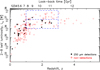 |
Fig. A.1. 2–8 keV X-ray luminosity vs. redshift for the sources in the CDF-N searched in 250 μm by SPIRE. The dashed lines enclose the LX = 1043 − 1044 erg s−1 and LX = 1044 − 1045 erg s−1 regions spanning z = 1 − 3 (cf. Fig. 1 in Page et al. 2012). The filled symbols show those detected in 250 μm emission (SFIR > 18 mJy), and unfilled for undetected, with the shapes representing the NED classification: stars for QSOs, circles for galaxies, and squares for unclassified. |
250 μm detection statistics above and below LX = 1044 erg s−1 (1037 W) for the LX = 1037 − 1039 W–z = 1 − 3 sample, the LX > 1035 W (> 1042 erg s−1) sample, and the whole sample (Page et al. 2012), in addition to the effect on each by including source number 40.
Following the SED fitting procedure described in Sect. 2.2, there is sufficient photometry to obtain the ionising photon rate for 103 of the CDF-N sources (Fig. A.2). The highest ionising photon rate at which 250 μm is detected is Q = 4.4 × 1055 s−1, which is consistent with the value above which H I 21 cm absorption remains undetected (Sect. 1). However, the p = 0.134 detection rate below this gives a binomial probability of P(bin)=0.137 for zero detections out of the 14 sources with Q > 4.4 × 1055 s−1, which is only significant at S(bin)=1.51σ. Moreover, when tested over a larger sample no critical rate is apparent (Sect. 3.1). Furthermore, extending the Page et al. (2012) sample, using the Chandra Deep Field South (CDF-S, Xue et al. 2011) and COSMOS fields (Elvis et al. 2009), finds no evidence for suppressed star formation at high X-ray luminosities (Harrison et al. 2012).
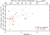 |
Fig. A.2. Ionising photon rate vs. redshift for the sources in the CDF-N. The symbols are as per Fig. A.1. |
All Tables
250 μm detection statistics above and below LX = 1044 erg s−1 (1037 W) for the LX = 1037 − 1039 W–z = 1 − 3 sample, the LX > 1035 W (> 1042 erg s−1) sample, and the whole sample (Page et al. 2012), in addition to the effect on each by including source number 40.
All Figures
|
Fig. 1. Distribution of the spectroscopic (filled histogram) and the photometric redshifts (unfilled) for the 62 073 matched SPIRE sources. |
| In the text | |
|
Fig. 2. Example of the FIR and UV photometry fits. The vertical line shows the observed-frame 250 μm frequency and the horizontal line the SPIRE confusion limit of 3σconf = 18 mJy. The shaded region shows the λ ≤ 912 Å band over which the ionising photon rate is derived. |
| In the text | |
|
Fig. 3. Distribution of spectral emissivity index and dust temperature, where Tdust ≤ 1.2 × 10¹²(z + 1)h/k, giving a sample of n = 2013. The shapes represent the NED classification: stars for QSOs, circles for galaxies, and squares for unclassified. |
| In the text | |
|
Fig. 4. Ionising (λ ≤ 912 Å) photon rate vs. redshift for the sources with spectroscopic redshifts. The filled symbols and histogram represent the FIR detections, unfilled for the non-detections. As in Fig. 3, the shapes represent the NED classification: stars for QSOs, circles for galaxies, and squares for unclassified. |
| In the text | |
|
Fig. 5. Dust temperature vs. ionising photon rate. Bottom panel: data are shown in equally sized bins. The horizontal bars show the range of points in the bin and the vertical error bars the 1σ uncertainty in the mean value. |
| In the text | |
|
Fig. 6. Dust temperature vs. total FIR luminosity. The dashed curve shows the fit for the SPIRE-mm sources (Roseboom et al. 2012). |
| In the text | |
|
Fig. 7. Dust temperature vs. the ionising photon rate normalised by the total FIR luminosity. |
| In the text | |
|
Fig. 8. Frequency of various stellar masses obtained from the initial mass function, ξ = ξ0Mα, normalised to give a total stellar mass of Mtotal = 4 × 10¹¹ M⊙, α = −0.3 for 0.01 < M⊙ < 0.08, α = −1.3 for 0.08 < M⊙ < 0.5, and α = −2.35 for M⊙ > 0.5 (Salpeter 1955; Kroupa 2001). The curve (right-hand scale) shows the approximate ionising photon rate per star. |
| In the text | |
|
Fig. 9. Far-IR luminosity distribution of the known QSOs and galaxies of the sample. |
| In the text | |
|
Fig. A.1. 2–8 keV X-ray luminosity vs. redshift for the sources in the CDF-N searched in 250 μm by SPIRE. The dashed lines enclose the LX = 1043 − 1044 erg s−1 and LX = 1044 − 1045 erg s−1 regions spanning z = 1 − 3 (cf. Fig. 1 in Page et al. 2012). The filled symbols show those detected in 250 μm emission (SFIR > 18 mJy), and unfilled for undetected, with the shapes representing the NED classification: stars for QSOs, circles for galaxies, and squares for unclassified. |
| In the text | |
|
Fig. A.2. Ionising photon rate vs. redshift for the sources in the CDF-N. The symbols are as per Fig. A.1. |
| In the text | |
Current usage metrics show cumulative count of Article Views (full-text article views including HTML views, PDF and ePub downloads, according to the available data) and Abstracts Views on Vision4Press platform.
Data correspond to usage on the plateform after 2015. The current usage metrics is available 48-96 hours after online publication and is updated daily on week days.
Initial download of the metrics may take a while.