| Issue |
A&A
Volume 627, July 2019
|
|
|---|---|---|
| Article Number | A10 | |
| Number of page(s) | 7 | |
| Section | The Sun | |
| DOI | https://doi.org/10.1051/0004-6361/201935629 | |
| Published online | 25 June 2019 | |
Long quasi-periodic oscillations of the faculae and pores
1
Tuorla Observatory, Department of Physics and Astronomy, University of Turku, Finland
e-mail: This email address is being protected from spambots. You need JavaScript enabled to view it.
2
Central (Pulkovo) Astronomical Observatory RAS, Pulkovskoe sh. 65, Saint-Petersburg, Russia
3
Saint-Petersburg State University, Universitetsky pr. 28, Saint-Petersburg, Russia
4
Kalmyk State University, Elista, Russia
Received:
5
April
2019
Accepted:
20
May
2019
Abstract
Aims. The main goal of this work is to analyze the structural and temporal evolution of small-scale magnetic structures (SSMSs) observed in the solar atmosphere, such as solitary faculae and pores, and reveal long quasi-periodic oscillations of these structures.
Methods. The statistical method of regression analysis and the wavelet transform were used to obtain the periods of oscillations and dependences between the parameters of magnetic structures and periods of oscillations.
Results. Long-period oscillations with periods in the interval of 18−260 min are found for the structurally stable phase of SSMSs at the level of the solar photosphere. These long-period oscillations were interpreted as natural oscillations of the structurally stable long-lived magnetic structures around their equilibrium position. These oscillations, which are of similar nature, are observed in the chromospheric bright formations associated with photospheric SSMSs. Dependences between the magnetic field and the continuum intensity of the facula elements were found. It is shown that the continuum intensity of a SSMS decreases when its magnetic field increases.
Key words: Sun: oscillations / Sun: magnetic fields / Sun: faculae / plages
© ESO 2019
1. Introduction
Recently, magnetohydrodynamic (MHD) oscillations of magnetic knots in the faculae regions of the Sun and the brightness variability of faculae visible in the solar chromosphere have been investigated very intensively, (e.g. Chelpanov et al. 2016; Kostik & Khomenko 2016). Bloomfield et al. (2006) and Jess et al. (2009) considered the physical connection between the bright points at the level of the chromosphere and the small-scale magnetic structures (SSMSs) at the level of photosphere. These authors found that different modes of MHD waves with periods in the interval of 3−5 min propagating upward along the magnetic field lines can transfer a great amount of energy up to the upper levels of the solar atmosphere. Some other structures with a magnetic field strength of the order of equipartition magnetic field (300−500 G) were studied by Martínez González et al. (2011). These latter authors found time variations of the magnetic field with periods compatible with the lifetime of granulation, or about 20 min. The result obtained for the pores by Freij et al. (2016) showed that periods of their oscillations were also enclosed in the range from 3 to 20 min. However, it should be noted that time series used in this latter study had the duration of about one hour only. Therefore any long-period oscillations would not have been revealed. A detailed description of MHD wave propagation and the current situation of the studies of oscillations in the photospheric SSMS were provided by Jess & Verth (2016).
The main goal of our study is the investigation of the long (with periods up to hundreds of minutes) quasi-periodic oscillations of the magnetic field of solitary faculae and pores (we also consider pores as SSMSs) when they have a structurally stable phase in their temporal evolution. The absolute value of magnetic field strength in these structures lies in the range from 200 to 1000 G. The typical cross-section size of these structures is 4−10 arcsec, and their lifetime varies from a few hours up to a few dozen hours. The faculae with a magnetic field smaller than 200 G have relatively short lifetimes, not more than two hours. For this reason, we did not include them in our research. Furthermore, we considered the mutual time variations of the average magnetic field of the structures mentioned above, and the average intensity of the bright chromospheric objects associated with these magnetic structures and located above them.
2. Observations and data processing
In order to analyze time variations of the magnetic field of the selected SSMSs, we used the full disk magnetograms for the line-of-sight component of magnetic field (“HMI_M_45, level 1”) obtained by the Helioseismic and Magnetic Imager (HMI) instrument on-board the Solar Dynamics Observatory (SDO) spacecraft (Schou et al. 2012; Scherrer et al. 2012).
We started with the magnetogram obtained on 06 July 2013 at 23:00:00 UT. All magnetograms considered in our study were obtained with a cadence of 45 s. In our work, the dates and times of observations were chosen randomly. The magnetic activity of the Sun was large enough for the small magnetic structures to be found. Furthermore, during the period from 5 to 7 July, 2013, we observed about five or six active regions on the solar disk with C-class flares. Therefore, on the first magnetogram we have selected 30 magnetic structures (pores and faculae) with the maximal value of the magnetic field strength in the range of 200−1000 G for both polarities. The typical spatial size of SSMSs on the magnetogram was found to be in the interval of 4−10 arcsec. All magnetic structures were selected far away from the mentioned active regions to avoid their possible influence on results. Each structure was fixed in a sliding box with a size of [15x15] pixels to perform a thorough analysis of its dynamical properties and trace its structural evolution in time.
Figure 1 shows an example of the time series obtained for the structure with the heliocentric coordinates [x, y]: [41, 664]; see also Table 1: structure with the number N = 4. The coordinates of these SSMSs on the solar surface were measured at 23:00:00 UT on 06 July 2013 (Table 1, column marked by [x; y]). Using such time series as shown in Fig. 1, we found the absolute value of maximal magnetic field strength (Bamax) for each magnetic structure (Table 1, column marked Bamax).
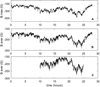 |
Fig. 1. Panel A: record of the maximal values of the magnetic field strength throughout the observation. Panel B: record of the average magnetic field strength of the observed magnetic structure. Panel C: record of the average values of the magnetic field for the morphologically quasi-stable phase of the magnetic “structure 4” in Table 1. |
Main characteristics of the small-scale magnetic structures.
A series of average values for the magnetic field (see Fig. 1, panels B and C) was determined via calculations of the magnetic field inside the contour of 50% of the maximal value of the magnetic field strength for each structure at each magnetogram. This series was used to obtain the periods of oscillations.
Furthermore, we used the HMI continuum filtergrams at 6173 Å, as well as EUV/UV data obtained for 304 Å, 1600 Å, and 1700 Å spectral passbands, which were observed with the Atmospheric Imaging Assembly (AIA) instrument on-board SDO (Lemen et al. 2012). The cadence of AIA 1600 Å and 1700 Å images is 24 s. This cadence is about two times shorter than the cadence of HMI magnetograms, that is, 45 s. Before the analysis, we binned up the cadence of AIA images to 48 s to minimize the inconvenience in comparing time-series. Thus, every second image was taken for the analysis. These images, with a cadence of 48 s, were taken at the same time interval as the magnetograms of HMI. On these images, we found bright structures associated with the selected magnetic structures. In agreement with the description of the considered spectral bands and the model of the solar atmosphere published by Avrett & Loeser (2008), we estimated that the emission at 1700 Å and 1600 Å originates at heights from 450 to 1500 km above the photosphere, and the emission at 304 Å originates over a wide range of chromospheric heights. The contours of 50% and 90% obtained from the magnetograms were then placed at the corresponding images obtained in the mentioned spectral passbands. A sample of such images for magnetic source 4 is presented in Fig. 2 (bottom). We calculated the average intensity for each considered structure in the EUV/UV images inside 50% contours. We used these average intensities to obtain the time series, which was then used to calculate the periods of brightness variations of the objects visible in the EUV/UV images.
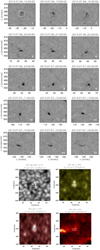 |
Fig. 2. Top: sample of typical structural evolution of magnetic “source 4” from Table 1 during the observations. Process of formation, the structurally stable phase, and the phase of destruction contain some consistent sets of images of the magnetic structure. The sequence number of the image is read from the left to the right and from the top to the bottom. Bottom: images obtained in different spectral bands with the contours of 50% and 90% of the magnetic field strength for “source 4”. |
To study the long quasi-periodic oscillations of the magnetic structures (pores and faculae) we need to define the time interval when the sources have well-formed structure and do not change their visible configuration, that is, the system retains its structural identity. We refer to this time interval as a structurally quasi-stable phase of SSMS and denote the duration of this phase as Tst (see also Table 1). The processes of the formation and the destruction of the magnetic structure are not directly related to the variation of the magnetic field during the time interval of Tst, because these processes have already finished or have not started yet (see Fig. 2, top). The top panel of Fig. 2 shows the process of formation of the morphologically stable SSMS and the process of its destruction and how these appear on the magnetograms. Figure 2 also shows the box (15 * 15) pixels (see image 1) inside which the SSMS was placed to trace its structural evolution. The first five images (1−5) represent the formation process of the magnetic structure. The next seven (6−12) images represent the structural quasi-stable phase (in the case of structure 4 shown in Fig. 2, this phase lasts about ten hours) and the last three images (13−15) represent the destruction process of the magnetic structure. Analyzing all sequential images (magnetograms) we have found the durations (Tst) of the structurally quasi-stable phase for all considered magnetic structures. It should be noted that the very small structural changes within a cadence of 45 s cannot be revealed visually with good accuracy. Therefore, for a reliable determination of the borders of Tst interval, we should trace the object over some period of time to be able to determine the small variations that result in the qualitative changes of the SSMSs. For that reason, the accuracy of the estimation of Tst is not better than 1 h.
3. Results
Using the time characteristics of SSMSs we built up the plot which shows how the duration of the structurally stable phase Tst depends on absolute maximal magnetic field strength Bamax. This plot is presented in Fig. 3 where the duration of the stable phase Tst is shown to have linear dependence on the absolute maximal magnetic field strength of the corresponding magnetic structures. This dependence was obtained by using the linear regression analysis. As one can see, the duration of the structurally stable phase grows with the increase of the absolute value of the magnetic field strength. The variance in the distribution of the parameters presented on the graph of Fig. 3 is significant because of the accuracy in determining Tst. Also, it should be noted that the absolute maximum magnetic field strength Bamax is not a reliable characteristic of the magnetic structure, because the magnetic field varies in time. Nevertheless, as seen from Fig. 3, this parameter has influence on the duration of the structurally stable phase of the structures.
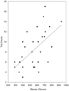 |
Fig. 3. Distribution of the Bamax vs. Tst of the considered SSMS. The solid line is the linear regression of the distribution. |
Generalized results obtained in this work are presented in Table 1. Column N gives the number of each of the considered magnetic structures. Column Pmag contains the values of the periods of quasi-periodic oscillations obtained from the variations of the average values of the magnetic field for the structural quasi-stable phase of the magnetic structures. Columns P1600; P1700; P304 give the values of the periods for the corresponding bright objects associated with the magnetic field structures.
Figure 4 shows the histogram for the periods obtained in our study. As one can see, the more common periods of the long oscillations of the SSMS are in the interval from 50 to 260 min. All these periods were obtained using the wavelet method suggested by Torrence & Compo (1998). The wavelet analysis is the most efficient method for studying quasi-periodicities in signals. It enables us to describe the behavior of a signal both in terms of time and frequency. In contrast to the wavelet method, which is restricted by an a priori assignment of harmonic basis functions, the Hilbert-Huang Transform (HHT) uses the empirical mode decomposition (EMD) of the signal of interest, iteratively searching for the local time-scale naturally appearing in the signal, and expands it into the basis derived directly from the data. Therefore, due to its adaptive nature, EMD is essentially suitable for the analysis of nonstationary and nonlinear variations. However, studies of the statistical significance of the obtained periodicities are more suitable for the wavelet method, and not for EMD. For this reason, we used traditional wavelet analysis in our study. In Table 1, the periods obtained with the wavelet method are presented. Values of the long periods are statistically significant (tested to the 95% significance level).
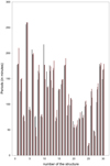 |
Fig. 4. Histogram of the periods of oscillations obtained for the thirty SSM structures. Bars obtained for the periods in the magnetic fields and in 1600 Å band are marked in black; bars obtained for the periods in 1700 Å and in 304 Å bands are marked in red. |
One sample of the wavelet analysis is shown in Fig. 5 (for the magnetic structure with serial number 4). We have taken into consideration only the periods which are statistically significant and have a maximal power as shown in the global wavelet panels.
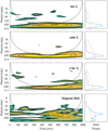 |
Fig. 5. Periods of the long quasi-periodic oscillations obtained by the wavelet method for the average magnetic field, and for the average intensities of the corresponding bright structures observed in different spectral passbands (in case of structure 4, Table 1). |
Figure 6 shows the simultaneous 1D profiles of the magnetic structures and the associated bright structures observed in different spectral passbands. As one can see, the location of the magnetic structure coincides with the locations of the associated bright structures seen in different spectral passbands (see also Fig. 2, bottom). Also, the maximal darkening visible in the continuum coincides with the position of the magnetic structure. If we assume that the magnetic field of SSMS has the cylindrical symmetry, then we can mark the variations of the diameter of the magnetic structure at different heights in the solar atmosphere. Simultaneously analyzing the profiles of images obtained in the spectral passbands 1600 Å and 1700 Å, which originate at heights of about 500−1500 km above the photosphere, with the profile of the magnetic field strength, we can say that beginning from the photosphere to the height of 500−1500 km the magnetic field lines of the considered structures do not diverge significantly. The profile obtained for the spectral band of 304 Å shows that in this case we have to deal with the diverged magnetic field lines at heights where this emission originates. This result is in relatively good agreement with the model of the SSMS presented by Jess & Verth (2016). Also, in Fig. 6 we see the magnetic field inclination of the structure resulting from the shifting of the maximal intensities obtained in the different spectral bands. We suppose this to be similar to the effect seen by Kobanov et al. (2015). We believe that the shifting of the positions of maximal intensity could lead to the small influence on the values of the periods derived for the considered SSM structures.
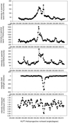 |
Fig. 6. One-dimensional profiles obtained simultaneously in different spectral bands for the magnetic field structure number 4 in Table 1. Positions of the associated brightness structures are seen in the corresponding boxes. |
Figure 7 shows the relation between the magnetic field strength and the intensity obtained in continuum observations of the magnetic structures. The values of the continuum intensity and the magnetic field strength were measured at the same time for all considered structures. A linear regression line in this plot is used to model the relationship between two variables by fitting a linear equation to measured data. It can be seen that brightness of the continuum for the considered SSMSs decreases with increasing magnetic field. A similar result was obtained for the contrast of the faculae and the magnetic bright points (MBPs) by Berger et al. (2007). The relative intensity of the continuum for the magnetic structures with weak magnetic field (in our case 200−400 G) is comparable to the quiet-sun level or slightly higher.
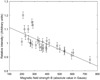 |
Fig. 7. Relation between the magnetic field strength and the relative brightness with the error bars of the small-scale magnetic structures seen in continuum observations. |
Results presented in Figs. 6 and 7 give us the numerical estimations of the intensity of small-scale chromospheric formations and how they depend on the magnetic fields. Also, they allow us to estimate both the sizes of the magnetic tubes at different heights in the solar atmosphere and the depth of the local brightness depression visible in the continuum.
Each graph in Fig. 8 contains a mutual distribution of parameters which are defined on the intersections of corresponding rows (four periods) and columns (Bamax and Tst). Also in the graphs, the regression line and the 95% confidence interval are presented. Therefore, Fig. 8 (column A) shows the dependences between the absolute maximal magnetic field strength and the periods of oscillations of these structures at different heights in the solar atmosphere. Figure 8 (column B) shows the dependences between the duration of the stable phase and the periods. From the panels (column A) we can see that relations between the absolute maximal magnetic field strength and the corresponding periods are relatively weak (correlation coefficients of about 0.23) in comparison with the relations shown in column B (correlation coefficients of about 0.86). Thus, the relations shown in column B between the duration of the stable phase and the corresponding periods observed at different heights are closer. Therefore, taking this result into account we can say that one of the most important parameters that define the long quasi-periodic oscillations of the SSMS is the duration of its structurally quasi-stable phase.
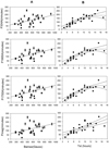 |
Fig. 8. Column A: dependences between Bamax (the absolute maximal magnetic field of the SMSS) and the periods Pmag, P1700 Å, P1600 Å, P304 Å (the oscillation periods with errors of the average magnetic field of the SMSS, and the periods of the intensities of the related structures obtained in the different spectral bands). Column B: relationships between Tst (the duration of the stable phase) and the periods Pmag, P1700 Å, P1600 Å, P304 Å. The errors are the same as in column A. |
In Fig. 9 the strong dependences between the periods of oscillations at different heights of the solar atmosphere are presented. The correlation coefficients for these cases are in the interval of 0.81−0.86. This allows us to suggest that in this case we observe the unified oscillatory process which was initiated by the oscillations of the magnetic structure as a whole. For all 30 magnetic structures considered in this work, we find that magnetic fields at the level of the photosphere have played an important role in the formation of the bright objects at different levels of the solar atmosphere. This means that bright structures which are visible in the different spectral bands are connected with the magnetic field of the corresponding SSMS. These magnetic fields define the very existence of these bright chromospheric formations.
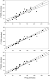 |
Fig. 9. Relation between the periods of the oscillations of the average magnetic field for the SSM structures and the periods obtained for the brightness structures at different spectral bands associated with the considered magnetic structures. The errors are the same as in column A of Fig. 8. |
4. Discussion and conclusions
Here we elucidate the long quasi-periodic oscillations of the SSMS. The periods of these oscillations were found to be in the interval from 50 to 260 min (see Table 1 and Fig. 4). We also showed that these periods depend on the duration of the structurally stable phase of the SSMS (see Fig. 8, column B). These oscillations penetrate to the heights where the emission of the considered spectral bands originates (see Fig. 9).
Recent studies provided by Strekalova et al. (2016) and Kolotkov et al. (2017) showed that SSMSs demonstrate oscillations in magnetic field strength with periods from tens of minutes up to 200−300 min. The authors of these latter studies suggested that long-period oscillations could be explained by the dynamical interaction between the magnetic structures and the boundaries of the surrounding super granules. However, the authors did not take into account the temporal evolution of the SSMS. Therefore, in this study we have tried to find one more reason for the existence of the long quasi-periodic oscillation of the faculae and the pores.
Three modes of nonlinear oscillations were revealed in an article by Solov’ev et al. (2019) devoted to the oscillations of facular knots. In this latter study, the EMD method suggested by Huang et al. (1998) was used for identification of the modes. The obtained results were interpreted on the basis of the facular knots model as a system with rigidity varying over time. In the present study, we apply the wavelet method despite its poor frequency resolution. However, frequency drift is clearly visible in Fig. 5 (wavelet for the magnetic field), which is typical for one of these modes, when the strength of the magnetic field falls, and the period of oscillations increases.
In our study, we do not make a clear distinction between faculae and small pores. Meanwhile, the inclusion of a small pore into the facular system increases its stability, and such stabilization can lead to the appearance of quasi-harmonic oscillations, a fourth mode, in addition to the three modes revealed in Solov’ev et al. (2019).
Such long-period oscillations are different from the relatively well-studied short-period oscillations of the SSMS. These short-period oscillations (in the interval from 3 to 15 min; see e.g. Thomas et al. 1984), are usually interpreted as the effect of the propagation of acoustic and MHD waves along the magnetic tube of the structure. Taking into account the typical size of the structures, we can say that such long oscillations cannot be explained by MHD wave propagation. Using results obtained in this study we conclude that SSMSs can be characterized by the absolute maximal magnetic field strength and the duration of the structurally quasi-stable phase Tst. In this phase, we observed a well-formed magnetic object, and thus we deal with the variation of the magnetic field of the well-formed structure as a whole. The duration of the stable phase of the system is much longer than the time of its relaxation to an equilibrium state. The latter can be estimated as the relation L/VA, where VA is the Alfven velocity and L is the typical size of the system in the scale from 4 to 10 arcsec. This means that the maximal size is about 7000 km. The Alfven velocity, even in the photosphere, is not less than VA = 106 cm s−1, in accordance with Murawski & Musielak (2010). Hence, the relaxation time is about a few minutes while the characteristic periods of the oscillations of the average magnetic fields and the intensities in the considered structures are measured in tens of minutes (see Table 1).
Therefore, we conclude that we have observed the stable magnetic structure which can oscillate as a whole near the state of its equilibrium. These oscillations should be considered as the natural oscillations of the system. The periods of such oscillations depend on the basic characteristics of the system: the magnetic field strength which determines the degree of its elasticity; the effective mass of gas (plasma) involved in these oscillations; and a number of parameters of the physical model (including the sizes of the magnetic tubes of the structure). Results presented in Fig. 9 allow us to conclude that these long quasi-periodic oscillations of the magnetic field propagate into the chromosphere and up to the transition region.
The local depressions of intensity (see Figs. 6 and 7) that are revealed here support the idea that long quasi-periodic oscillations can be regarded as natural oscillations of the SSMS in analogy with the mentioned model of sunspots. We draw special attention to the problem of intensity depression of SSMSs observed in continuum, because we assume that the physical structure of a facular knot is similar to the structure of a sunspot. According to the model of a shallow sunspot, Wilson’s depression, along with the cooling of the spot plasma, plays an important role in ensuring the stability of the system due to reducing its gravitational energy. The sunspot comes to a state of stable equilibrium and oscillates as a whole singular magnetic structure near the equilibrium with the periods of 10−30 h in accordance with Efremov et al. (2018). We assume that a similar effect takes place in the facular structures, and therefore the signatures of Wilson’s depression in facular elements especially attract our attention. The most important result of the work is the establishment of a direct relationship between the intensity of the magnetic element in the continuum and the magnetic field strength: as the field grows from the equipartition level (200−300 G) to the strength of 800 G, the intensity of the facular element at the level of the photosphere drops by 15%. In a future study, we would like to use more magnetic sources with field strengths in the interval from 200 to 1300 G to provide more reliable relations for the physical model of SSMSs (like facular knots and pores) and try to find analogies with the “shallow sunspot” model.
Acknowledgments
Authors thank the team of SDO for the possibility of using materials of the Solar Dynamic Observatory. Solov’ev A.A. was partially supported by Russion Scientific Foundation grant 15-12-20001, and Russian Foundation for Basic Research (RFBR) grant 18-02-00168. Smirnova V.V. was supported by Russion Scientific Foundation grant 16-12-10448. Strekalova P.V. and Zhivanovich I. were supported by Russian Foundation of Basic Research grant 18-32-00555 (mol_a).
References
- Avrett, E. H., & Loeser, R. 2008, ApJS, 175, 229 [NASA ADS] [CrossRef] [Google Scholar]
- Berger, T. E., Rouppe van der Voort, L., & Löfdahl, M. 2007, ApJ, 661, 1272 [NASA ADS] [CrossRef] [Google Scholar]
- Bloomfield, D. S., McAteer, R. T. J., Mathioudakis, M., & Keenan, F. P. 2006, ApJ, 652, 812 [NASA ADS] [CrossRef] [Google Scholar]
- Chelpanov, A. A., Kobanov, N. I., & Kolobov, D. Y. 2016, Sol. Phys., 291, 3329 [NASA ADS] [CrossRef] [Google Scholar]
- Efremov, V. I., Solov’ev, A. A., Parfinenko, L. D., et al. 2018, Ap&SS, 363, 61 [NASA ADS] [CrossRef] [Google Scholar]
- Freij, N., Dorotovič, I., Morton, R. J., et al. 2016, ApJ, 817, 44 [NASA ADS] [CrossRef] [Google Scholar]
- Huang, N. E., Shen, Z., Long, S. R., et al. 1998, Proc. R. Soc. London Ser. A, 454, 903 [NASA ADS] [CrossRef] [Google Scholar]
- Jess, D. B., & Verth, G. 2016, Geophysical Monograph Series (Washington, DC: American Geophysical Union), 216, 449 [CrossRef] [Google Scholar]
- Jess, D. B., Mathioudakis, M., Erdélyi, R., et al. 2009, Science, 323, 1582 [NASA ADS] [CrossRef] [PubMed] [Google Scholar]
- Kobanov, N., Kolobov, D., & Chelpanov, A. 2015, Sol. Phys., 290, 363 [NASA ADS] [CrossRef] [Google Scholar]
- Kolotkov, D. Y., Smirnova, V. V., Strekalova, P. V., Riehokainen, A., & Nakariakov, V. M. 2017, A&A, 598, L2 [NASA ADS] [CrossRef] [EDP Sciences] [Google Scholar]
- Kostik, R., & Khomenko, E. 2016, A&A, 589, A6 [NASA ADS] [CrossRef] [EDP Sciences] [Google Scholar]
- Lemen, J. R., Title, A. M., Akin, D. J., et al. 2012, Sol. Phys., 275, 17 [NASA ADS] [CrossRef] [Google Scholar]
- Martínez González, M. J., Asensio Ramos, A., Manso Sainz, R., et al. 2011, ApJ, 730, L37 [NASA ADS] [CrossRef] [Google Scholar]
- Murawski, K., & Musielak, Z. E. 2010, A&A, 518, A37 [NASA ADS] [CrossRef] [EDP Sciences] [Google Scholar]
- Scherrer, P. H., Schou, J., Bush, R. I., et al. 2012, Sol. Phys., 275, 207 [Google Scholar]
- Schou, J., Scherrer, P. H., Bush, R. I., et al. 2012, Sol. Phys., 275, 229 [Google Scholar]
- Solov’ev, A. A., Strekalova, P. V., Smirnova, V. V., & Riehokainen, A. 2019, Ap&SS, 364, 29 [NASA ADS] [CrossRef] [Google Scholar]
- Strekalova, P., Nagovitsyn, Y. A., Riehokainen, A., & Smirnova, V. 2016, Geomag. Aeron., 56, 1 [CrossRef] [Google Scholar]
- Thomas, J. H., Cram, L. E., & Nye, A. H. 1984, AJ, 285, 368 [NASA ADS] [CrossRef] [Google Scholar]
- Torrence, C., & Compo, G. P. 1998, Am. Meteorol. Soc., 79, 61 [NASA ADS] [CrossRef] [Google Scholar]
All Tables
All Figures
|
Fig. 1. Panel A: record of the maximal values of the magnetic field strength throughout the observation. Panel B: record of the average magnetic field strength of the observed magnetic structure. Panel C: record of the average values of the magnetic field for the morphologically quasi-stable phase of the magnetic “structure 4” in Table 1. |
| In the text | |
|
Fig. 2. Top: sample of typical structural evolution of magnetic “source 4” from Table 1 during the observations. Process of formation, the structurally stable phase, and the phase of destruction contain some consistent sets of images of the magnetic structure. The sequence number of the image is read from the left to the right and from the top to the bottom. Bottom: images obtained in different spectral bands with the contours of 50% and 90% of the magnetic field strength for “source 4”. |
| In the text | |
|
Fig. 3. Distribution of the Bamax vs. Tst of the considered SSMS. The solid line is the linear regression of the distribution. |
| In the text | |
|
Fig. 4. Histogram of the periods of oscillations obtained for the thirty SSM structures. Bars obtained for the periods in the magnetic fields and in 1600 Å band are marked in black; bars obtained for the periods in 1700 Å and in 304 Å bands are marked in red. |
| In the text | |
|
Fig. 5. Periods of the long quasi-periodic oscillations obtained by the wavelet method for the average magnetic field, and for the average intensities of the corresponding bright structures observed in different spectral passbands (in case of structure 4, Table 1). |
| In the text | |
|
Fig. 6. One-dimensional profiles obtained simultaneously in different spectral bands for the magnetic field structure number 4 in Table 1. Positions of the associated brightness structures are seen in the corresponding boxes. |
| In the text | |
|
Fig. 7. Relation between the magnetic field strength and the relative brightness with the error bars of the small-scale magnetic structures seen in continuum observations. |
| In the text | |
|
Fig. 8. Column A: dependences between Bamax (the absolute maximal magnetic field of the SMSS) and the periods Pmag, P1700 Å, P1600 Å, P304 Å (the oscillation periods with errors of the average magnetic field of the SMSS, and the periods of the intensities of the related structures obtained in the different spectral bands). Column B: relationships between Tst (the duration of the stable phase) and the periods Pmag, P1700 Å, P1600 Å, P304 Å. The errors are the same as in column A. |
| In the text | |
|
Fig. 9. Relation between the periods of the oscillations of the average magnetic field for the SSM structures and the periods obtained for the brightness structures at different spectral bands associated with the considered magnetic structures. The errors are the same as in column A of Fig. 8. |
| In the text | |
Current usage metrics show cumulative count of Article Views (full-text article views including HTML views, PDF and ePub downloads, according to the available data) and Abstracts Views on Vision4Press platform.
Data correspond to usage on the plateform after 2015. The current usage metrics is available 48-96 hours after online publication and is updated daily on week days.
Initial download of the metrics may take a while.