| Issue |
A&A
Volume 625, May 2019
|
|
|---|---|---|
| Article Number | A81 | |
| Number of page(s) | 13 | |
| Section | Interstellar and circumstellar matter | |
| DOI | https://doi.org/10.1051/0004-6361/201935309 | |
| Published online | 16 May 2019 | |
Photodissociation of CO in the outflow of evolved stars
Department of Space, Earth and Environment, Chalmers University of Technology,
Onsala Space Observatory,
43992
Onsala,
Sweden
e-mail: maryam.saberi@chalmers.se
Received:
19
February
2019
Accepted:
25
March
2019
Context. Ultraviolet (UV) photodissociation of carbon monoxide (CO) controls the abundances and distribution of CO and its photodissociation products. This significantly influences the gas-phase chemistry in the circumstellar material around evolved stars. A better understanding of CO photodissociation in outflows also provides a more precise estimate of mass-loss rates.
Aims. We aim to update the CO photodissociation rate in an expanding spherical envelope assuming that the interstellar radiation field (ISRF) photons penetrate through the envelope. This will allow us to precisely estimate the CO abundance distributions in circumstellar envelope around evolved stars.
Methods. We used the most recent CO spectroscopic data to precisely calculate the depth dependency of the photodissociation rate of each CO dissociating line. We calculated the CO self- and mutual-shielding functions in an expanding envelope. We investigated the dependence of the CO profile on the five fundamental parameters mass-loss rate, the expansion velocity, the CO initial abundance, the CO excitation temperature, and the strength of the ISRF.
Results. Our derived CO envelope size is smaller than the commonly used radius derived by Mamon et al. (1988, ApJ, 328, 797). The difference between results varies from 1 to 39% and depends on the H2 and CO densities of the envelope. We list two fitting parameters for a large grid of models to estimate the CO abundance distribution. We demonstrate that the CO envelope size can differ between outflows with the same effective content of CO, but different CO abundance, mass-loss rate, and the expansion velocity as a consequence of differing amounts of shielding by H2 and CO.
Conclusions. Our study is based on a large grid of models employing an updated treatment of the CO photodissociation, and in it we find that the abundance of CO close to the star and the outflow density both can have a significant effect on the size of the molecular envelope. We also demonstrate that modest variations in the ISRF can cause measurable differences in the envelope extent.
Key words: astrochemistry / stars: AGB and post-AGB / circumstellar matter / stars: abundances / ultraviolet: stars / molecular processes
© ESO 2019
1 Introduction
Asymptotic giant branch (AGB) stars are among the most important contributors of dust and heavy elements in the universe. These stars enrich the interstellar medium (ISM) and galaxies by ejecting a large fraction of their material through strong stellar winds. An extended circumstellar envelope (CSE) will be created around the star as a consequence of the intense mass loss (e.g. Habing & Olofsson 2003). Understanding the complex chemical networks in the CSE of AGB stars is required for a better understanding of the enrichment and chemical evolution of the ISM and galaxies.
Carbon monoxide (CO), the most abundant molecule after molecular hydrogen (H2), has been used to constrain the physical properties and chemical composition of the ISM and CSEs (e.g. Goldreich & Scoville 1976; Scalo & Slavsky 1980; Millar et al. 1987; Garrod & Herbst 2006; Morata & Herbst 2008). Photodissociation by ultraviolet (UV) radiation is the dominant process destroying CO and determining its abundance distribution. Therefore, a precise estimation of the CO photodissociation rate is important in both chemical and physical modelling of CSEs.
Generally speaking, molecular photodissociation by UV radiation can dominate by direct or indirect photodissociation, depending on the molecular structure. In direct photo-dissociation, the photodissociation cross section is continuous as a function of photon energy (continuum photodissociation). Thus, all absorptions lead to molecular dissociation. For indirect photodissociation, the photodissociation cross section contains a series of discrete peaks (line photodissociation). Therefore, absorption at only certain wavelengths leads to molecular dissociation. At wavelengths shorter than that of the H Lyman limit (911.7 Å), CO photodissociation occurs entirely in a set of discrete UV wavelength lines. This process makes CO strongly subject to self shielding, in cases of high abundance, and to mutual shielding by other species which are dissociated at the same wavelengths such as atomic and molecular hydrogen, atomic carbon, and dust. The dissociating photons will be absorbed by species closer to the UV source and thus molecules at the deeper regions will be shielded. The amount of shielding depends on the UV intensity, the geometry of the cloud which determines the photon penetration probability, and the column density of species with the same dissociating wavelengths. Bally & Langer (1982) and Glassgold et al. (1985) have shown the importance of the CO self-shielding in molecular clouds based on anomalous intensity ratios of various CO isotopologues which are selectively photodissociated in the edge of molecular clouds due to various column densities.
The most updated CO unshielded photodissociation rate in the interstellar medium of the solar neighborhood is estimated to be 2.6 × 10⁻¹⁰ s−1 by Visser et al. (2009). We derive the same unshielded photodissociation rate in the outflows of evolved stars assuming that the Draine (1978) radiation field penetrates the envelope. This rate depends only on the following: the radiation field, the accuracy of the CO spectroscopic data and the surface temperature of the astrophysical region.
However, the geometrical distances over which the photodissociation is significant depends strongly on the physicalconditions of the penetrated environment such as its geometry, temperature distribution, and H2 density. Thus, the environmental properties should be taken into account in calculations of the self- and mutual-shielding functions in various environment such as interstellar clouds and CSEs.
There is a good understanding of the depth dependency of the CO photodissociation mechanism in interstellar clouds and the photodissociation rate has been regularly updated with new laboratory data (e.g. Solomon & Klemperer 1972; Bally & Langer 1982; Glassgold et al. 1985; van Dishoeck & Black 1986, 1988; Visser et al. 2009). The shielding functions for several sets of input parameters for interstellar clouds can be downloaded1 from the work by Visser et al. (2009).
In case of CSEs, Morris & Jura (1983, hereafter MJ83) present the theory of calculating the depth dependency of the CO photodissociation rate by considering CO self-shielding and H2 mutual-shielding in a spherical expanding envelope through a “one-band approximation”. In this approximation, they assume that CO dissociates only at 1000 Å. After higher resolution laboratory measurement of far-UV absorption and fluorescence cross sections by Letzelter et al. (1987), the rate was updated by Mamon et al. (1988, hereafter MGH88) considering 34 dissociating-bands. Afterwards, Visser et al. (2009) collected the latest CO laboratory measurements of 855 UV dissociating lines arising in levels J = 0–9 in the lowest vibrational state v = 0. The updated CO photodissociation rate in a CSE is presented in two recent works by Li et al. (2014) and Groenewegen (2017). However, both works use the shielding functions calculated for an interstellar cloud (Visser et al. 2009) not a CSE. In the current work, we aim to calculate the CO photodissociation rate in a CSE using the most updated laboratory data and following the shielding functions developed for CSEs by MJ83 and MGH88. We discuss the differences of the depth dependency of the photodissociation rate in interstellar clouds and CSEs in Sect. 4.3. In addition, we have investigated the effect of several more free parameters on the CO dissociation rate. The new treatment of the CO photodissociation has been incorporated into a chemical network describing the CSEs of AGB stars.
2 Circumstellar chemistry
We use an extended version of the publicly available circumstellar envelope chemical model rate13-cse code2 (McElroy et al. 2013). We modified calculations of the CO photodissociation rate from a one-band approximation to a treatment where all known lines are taken into consideration (see Sect. 2.2).
The code assumes a spherically symmetric envelope which is formed due to a constant mass loss Ṁ. The envelope expands with a constant radial velocity Vexp. The H2 density falls as 1∕r2 where r measures the distance from the central star. We used the gas temperature profile given by MGH88 which is derived for CW Leo as follows:
 (1)
(1)
where r0 = 9 × 1016 cm, β = 0.72 for r < r0 and β = 0.54 for r > r0. We assume a minimum temperature of 10 K in the outer CSE.
We incorporated an extended version of the chemical network from the UMIST Database for Astrochemistry (McElroy et al. 2013) which includes the 13C and 18O isotopes, all corresponding isotopologues, their chemical reactions and the properly scaled reaction rate coefficients (Röllig & Ossenkopf 2013). The chemical network includes 933 species and 15108 gas-phase reactions. The isotopologue chemistry will be discussed in detail in a forthcoming paper.
2.1 CO spectroscopic data
The dissociation energy of the CO ground state is 11.09 eV, thus the photodissociation occurs in the wavelength range 911.75–1117.8 Å. The CO photodissociation occurs entirely through line absorptions into pre-dissociating states (e.g. Visser et al. 2009). We use the latest laboratory measurements of CO data (Visser et al. 2009) which includes 855 UV transitions containing rotational excitations J = 0−9 to calculate the photodissociation rate. The higher excitation levels up to J = 30 were examined in the calculations and since the effect was marginal, we excluded the higher transitions to increase the time efficiency of the code.
2.2 CO photodissociation rate
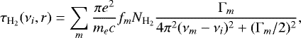
The total CO photodissociation rate at radius r is the summation of the photodissociation rates of all discrete contributing lines i as follows:
 (2)
(2)
where  is the CO unshielded photodissociation rate at the edge of the cloud, βi counts the CO self-shielding efficiency and γi counts the mutual shielding from other species.
  is estimated to be 2.6 × 10⁻¹⁰ s−1 and the detailed calculations are presented in the Appendix A.1. We note that in calculations of the photodissociation rates we assumed the CO excitation temperature Tex to be the same as the gas kinetic temperature Tkin given in Eq. (1).
Dissociating radiation can be absorbed by CO (self-shielding), H, C, H2 and dust (mutual-shielding) (e.g. MGH88; Visser et al. 2009). The mutual shielding by different species depends on their column density and the amount of line overlaps in the relevant region of the spectrum. The amount of mutual shielding by dust is assumed to depend on the total number of protons [n(H)+2n(H2)] which determine the dust extinction. In our models, the column densities of C and H are insufficient to produce very much blocking. Thus, the shielding by dust and H2 dominates the CO mutual shielding. We note that in the presence of extra UV radiation from a hot binary companion and/or stellar chromospheric activity there could be an enhancement of the atomic abundances. The investigation of how and whether these would impact the CO abundance distribution is, however, beyond the scope of the current study.
Calculations of the depth dependency of the CO photodissociation rate require accurate information on the line wavelength, oscillator strengths, the pre-dissociation probabilities and the line widths of CO and H2. We used the new compiled H2 line list (J. Black, priv. comm.) based on energy levels and transition probabilities computed by Abgrall et al. (1994, 1997). In the Appendix A, we review the underlying physics of calculations of shielding functions β and γ in an expanding CSE.
Envelope parameters and assumptions for the reference model.
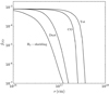 |
Fig. 1 CO fractional abundance distributions for simulations with different shielding functions that regulate CO photodissociation: shielding by H2, shielding by dust, CO self-shielding, and the total shielding for the reference model. |
3 Results
To study the significance of the different shielding processes we use a reference model with the physical parameters listed in Table 1. This model serves as a direct comparison to the work by MGH88. Figure 1 shows the fractional CO abundance profile calculated by considering different shielding contributions from CO, H2, dust, and the total shielding for the reference model. As we can see, the CO self-shielding plays a major role in the total shielding.
In Fig. 2 we illustrate how the CO abundance distribution varies for models with different initial CO abundances f0 and mass-loss rates Ṁ while preserving the total amount of CO ejected by the star. It is clear that the H2 density (set by Ṁ and Vexp) dictates the size of the envelope, while the initial CO abundance affects the steepness of the slope. This differentiation provides a way to break the degeneracy between fCO and Ṁ encountered when both low-J and high-J CO transitions are used in CO radiative transfer (RT) modelling.
Figure 3 presents the variation of the CO distribution profiles with Ṁ, keeping all other parameters the same as the reference model. An increase in Ṁ translates into a stronger shielding and hence a larger CO envelope with a sharper drop-off at the outer edge.
The CO abundance profiles derived from our simulations can be fitted by the analytical formula derived by MGH88 as follows:
 (3)
(3)
where f0 is the initial CO abundance, α determines the steepness of the profile and r1∕2 marks the radius where the CO abundance drops to half of its initial value. Figure 4 shows the accuracy of the fitting formula for a range of mass-loss rates; all other parameters are the same as the reference model given in Table 1. In general, f0 depends on the chemical type of AGB star and is commonly assumed to have average values (2 − 6 − 10) × 10−4 for M-, S-, and C-type AGB stars, respectively (Ramstedt & Olofsson 2014).
We derive α and r1∕2 for a grid containing 390 models with varying f0, Ṁ, and Vexp. We considered ten values for f0 (1, 2, ⋯, 10 × 10−4), 13 values for Ṁ ([1, 2, 5] ×10−8, [1, 2, 5] × 10−7, …, 1 × 10⁻⁴ M⊙ yr−1), and three values for Vexp (7.5, 15, 30 km s−1). Table B.1 lists the resulting α and r1∕2 values for all models. Figure 5 shows how variations of fCO, Ṁ, and Vexp affect α and r1∕2. Increasing Ṁ and decreasing Vexp leads to an enhancement of the  and thus more shielding and a larger CO envelope. Similarly an increase in fCO enhances the CO self-shielding. The most drastic changes in α and r1∕2 happen for oxygen-type AGB stars with lower CO abundance, where the CO self-shielding is not very efficient.
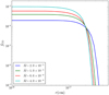 |
Fig. 2 CO fractional abundance distributions for models with a constant expansion velocity Vexp = 15 (km s−1) and various Ṁ (M⊙ yr−1) and fCO in a way to keep the same amount of effective CO for all models. |
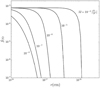 |
Fig. 3 CO fractional abundance distributions for models with fCO = 8 × 10⁻⁴, Vexp = 15 (km s−1), and a range of mass-loss rates which are marked in the figure. |
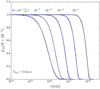 |
Fig. 4 Comparison of the CO fractional abundance distributions from modelling (solid black lines) and the analytic fitting formula (dashed blue lines) for models with fCO = 8 × 10⁻⁴, Vexp = 15 (km s−1) and a range of 10−8 < Ṁ < 10−4 (M⊙ yr−1). |
4 Discussion
4.1 Influence of the temperature on the CO abundance distribution
We examined the influence of the gas kinetic temperature profile on the CO envelope size for the reference model. The CO excitation temperature is assumed to be the same as the gas kinetic temperature profile which is given in Eq. (1). We assumed the temperature and radius at the inner envelope to be T0 = 2000 K and r0 = 1014 cm. We considered 0.4 < β < 1.0 which reasonably covers the gas temperature profile of AGB CSEs (De Beck et al. 2012; Danilovich et al. 2014; Khouri et al. 2014; Maercker et al. 2016; Ramos-Medina et al. 2018; Van de Sande et al. 2018). β determines the slope of the profile. Figure 6 shows the considered temperature profiles and their corresponding CO abundance distributions. The fitting parameters vary in the ranges 1.65 × 10¹⁷ < r1∕2 < 2.03 × 1017 cm and 3.00 < α < 3.24. The temperature profiles with β ≥ 0.6 give rise to similar CO abundance distributions whereas those with β < 0.6 lead to smaller envelopes. This is due to a lower shielding effectiveness in the hotter envelope (see Appendix A).
We also examined the influence of constant CO excitation temperature Tex = 5, 20, 50, 100 K as assumed by Groenewegen (2017) versus Tex = Tkin for the reference model. The two fitting parameters vary in ranges 1.53 × 10¹⁷ < r1∕2 < 2.25 × 1017 cm and 2.88 < α < 3.41. As shown in Fig. 7 a lower CO excitation temperature results in a bigger CO envelope. The reduced Tex leads to higher lower-level populations xl (see Appendix A) and thus more efficient shielding and therefore a bigger envelope.
4.2 Influence of the ISRF on the CO abundance distribution
The Draine interstellar radiation field (ISRF) that we considered in this work has been measured in the solar neighborhood. McDonald & Zijlstra (2015) show that the ISRF is considerably higher in globular clusters. This will have a significant impact on the size of the CO envelope of evolved stars which are located in clusters (McDonald et al. 2015). On the other hand, objects which lie above the Galactic plane, for example IRC+10216, are possibly exposed to a weaker ISRF. We investigated the influence of the strength of the ISRF on the CO envelope size. We scaled the Draine (1978) radiation field that we used for the reference model by factors χ = 0.25, 0.5, 1, 2, and 4. Table 2 presents the results for models with the mass-loss rates Ṁ = 10−8, 10−7, 10−6, 10−5, 10−4 M⊙ yr−1. We considered the expansion velocity Vexp = 15 km s−1 and the initial CO abundance of fCO = 8 × 10⁻⁸ for all models. As expected, the effect of the ISRF strength on the CO envelope size is more prominent in stars with low mass-loss rates with weaker shielding efficiency. Increasing the ISRF by a factor of two reduces the CO envelope size by 40, 34, 28, 20, 14% for stars with Ṁ = 10−8, 10−7, 10−6, 10−5, 10−4 M⊙ yr−1, respectively.
We notethat in some cases, there is extra UV radiation which internally penetrates into the CSE. The inner UV radiation can arises from stellar chromospheric activity and/or a hot binary companion (e.g. Montez et al. 2017). In hot post-AGB stars, the high temperature of the star itself also generates UV photons. In such cases, the inner UV radiation will be quickly absorbed by inner dust and thus is not expected to affect the extent of the CO envelope. However this likely affects the CSE chemistry (e.g. Saberi et al. 2017, 2018; Van de Sande & Millar 2019) in the dust formation region, which is beyond the scope of this paper.
4.3 Environmental dependency of the CO photodissociation rate
The differences in the physical and chemical properties between interstellar clouds and CSEs can affect the CO shielding functions and thus the depth dependency of CO photodissociation rates. Here we list the environmental differences between interstellar clouds (Visser et al. 2009) and CSEs (this work) that enter in calculations of shielding functions:
- (a)
Model geometry: in interstellar cloud models, plane-parallel geometry has been considered while in the CSE model spherically symmetric geometry is assumed. The difference in the geometry affects the photon penetration probability.
- (b)
CO excitation temperature: a constant temperature that can be chosen among the values of 5, 20, 50 and 100 K is available in interstellar clouds model. In the modelling of the CSE, we consider Tex (CO) to be the same as Tkin which varies in a range ~10−2000 K. This affects the fractional population of the lower-level especially in the inner CSE. Assuming a too low Tex leads to an overestimation of the CO self-shielding as shown in Fig. 7.
- (c)
Atomic and molecular line broadening: the Doppler and natural broadenings are the dominant processes which control the CO, H2 and H line widths in the interstellar clouds. Since the CSE around AGB stars is expanding at velocities of typically a few up tosome 30 km s−1, the expansion velocity should also be considered in the calculations of the line widths.
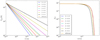 |
Fig. 6 Left panel: tested gas kinetic temperature profiles with different β values. Theprofile with label “reference” corresponds to the temperature of the reference model. Right panel: CO abundance distribution profile derived using the temperature profiles from the left panel. |
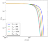 |
Fig. 7 CO fractional abundances distributions for the reference model when different CO excitation temperature profiles are considered in calculations of the CO photodissociation rate. |
Fitting parameters of the CO envelope size for a range of ISRF intensity.
4.4 Comparison with literature
The most commonly used method to derive the size of the CO envelope is the one presented by MGH88. They used the Jura (1974) radiation field to calculate the CO photodissociation rate. The Jura radiation field in addition to more UV observations at longer wavelengths up to 2000 Å has been later used by Draine (1978) to derive an analytical formula for the standard ISRF (Lee 1984). Thus, in principle in the wavelength range 930–1125 Å, both Draine and Jura radiation fields represent the same UV observational data. MGH88 presented the fitting parameters of the CO envelope size for a grid of models with a constant CO abundance of 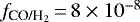 and 13 varying mass-loss rates and three expansion velocities. However, in addition to now outdated low-resolution CO laboratory data which causes underestimation of the unshielded photodissociation rate by 30%, a major drawback of this work is that it is based on calculations that assume one fixed value of f0 = 8 × 10⁻⁴. We clearly demonstrate in the previous section that the role of f0 is non-negligible in the overall dissociation efficiency. Table 3 and Fig. 8 compare the MGH88 results for the r1∕2 and α fitting parameters with those derived in this work. The difference in fitting parameters ranges from 0.6 to 15% for α and 1 to 39% for r1∕2 between two works. In almost all tested cases, our models predict the steepness parameter α to be larger than that derived by MGH88, indicating a less efficient shielding of CO in our study. In line with this, we calculate consistently smaller values for r1∕2. This is consistent with observational data for W Hya (Khouri et al. 2014), TX Cam (Ramstedt et al. 2008), and R Dor (Maercker et al. 2016) for example. Models of these objects reproduce the observed line emission better when they assume a smaller CO envelope than is predicted by MGH88, in line with the results of this paper.
Our derived CO radius is also smaller by 11–60% compared to Groenewegen (2017) depending on the H2 density of the envelope. This comes from different shielding functions used to calculate the depth-dependent CO photodissociation rate.
4.5 Predicting the CO line fluxes
We have tested the effect of CO abundance profiles derived in this work and by MGH88 on the CO line intensities for two models in Table 3. We use a non-local thermodynamic equilibrium (non-LTE) RT code based on the Monte Carlo programme (see e.g. Schöier & Olofsson 2001) for the excitation analysis.
Model 1. The first model is the reference model with its CSE properties are given in Table 1. We assumed that the reference star is at a distance of 1 kpc in order to cover the entire envelope with a 12-m telescope beam. The fitting parameters of the CO envelope size are r1∕2 = 2.02 × 1017 cm and α = 3.10 from this work and r1∕2 = 2.35 × 1017 cm and α = 2.79 from MGH88. Figure 9 presents the results of RT modelling for CO(1–0, 2–1, 3–2) transitions for this model. The 14% difference in r1∕2 size only becomes visible in J = 1−0 spectrum in this case. We find a 5% difference in the total intensity of J = 1−0 transition which is less than the commonly assumed 20% uncertainty of single-dish observations. However, comparing the integrated intensity at radial offset points from the central star shows bigger discrepancy between two models. The differences in the integrated intensity at distance 22″ = 3.2 × 1017 cm reaches to 34%. This indicates that CO high-resolution observations which provide the integrated intensity at radial offset points are more powerful to constrain photodissociation models.
Model 2. We selected the model with the biggest discrepancy with MGH88 work. This model has Ṁ = 10−4 M⊙ yr−1 and Vexp = 7.5 km s−1. The star is assumed to be at distance of 3 kpc from the earth to cover the entire envelope with a 12-m telescope beam. The fitting parameters of the CO envelope size are r1∕2 = 9.91 × 1017 cm and α = 3.80 from this work and r1∕2 = 1.64 × 1018 cm and α = 3.71 from MGH88. Figure 10 shows the results of the CO RT modelling for these two models. The clearest difference is again apparent for CO(1–0), where the emission is substantially different in the velocity range [−10,−5] km s−1. In the blue model, the emission is entirely self-absorbed. This can be explained by the absence of a significant amount of cold CO gas in the red model, which is characterised by a smaller r1∕2 than the blue model. For this model, the integrated intensities at radial offset points of the red model (this work) are higher due to the absorption in the blue model (MGH88).
Comparison of the fitting parameters of the CO envelope between this work and MGH88.
5 Summary
We have presented detailed calculations of the CO photodissociation rate in a spherically symmetric CSE which is expanding with a constant velocity. The standard Draine (1978) radiation field is assumed to penetrate into the CSE from all directions. We used the latest CO spectroscopic data to calculate the shielding functions. We examined the impact of variation of five primary important factors Ṁ, Vexp, fCO, Tex (CO), and the strength of the ISRF χ on the CO abundance distributions. The effect of varying parameters on the CO envelope size is more prominent for either low-mass loss stars or the ones with low initial CO abundance. This can be explained by lower shielding efficiency.
Assuming the same ISRF and CSE properties, our derived CO envelope size is smaller than the commonly used radius presented by MGH88. We show that having the same amount of effective CO with a different set of physical parameters does not necessarily give the same CO abundance distribution. High-resolution ALMA observations, for example the DEATHSTAR3 project (Ramstedt et al. In prep), can, together with our new formalism of determination of the CO envelope size, be used to decrease theuncertainty in mass-loss determinations.
Although we listed two fitting parameters of the CO abundance distribution for a large grid of models, it is recommended to run models for individual stars separately considering their individual physical parameters. Moreover, we strongly recommend running optimised models in case there are clear indications for a locally weak or strong ISRF based on other observations.
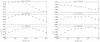 |
Fig. 8 Comparison of CO abundance distribution parameters to MGH88 results. The left panel shows
|


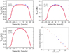 |
Fig. 9 Results of CO RT modelling for model 1 (the reference model) with the CO abundance distribution from this work (red) and MGH88 (blue). The transitions and the beam size are marked in each panel. Bottom right panel: compares the radial distribution of the CO(1–0) integrated intensities at radial offset points. |
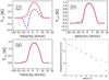 |
Fig. 10 Results of CO RT modelling for model 2 with extreme discrepancy between the CO abundance distribution from this work (red) and MGH88 (blue). The transitions and the beam size are marked in each panel. The bottom right panel compares the radial distribution of the CO(1–0) integrated intensities at radial offset points. |
Acknowledgements
This work was supported by ERC consolidator grant 614264. E.D.B. acknowledges financial support from the Swedish National Space Agency. We thank John Black for fruitful discussions on the detailed calculations of photodissociation rates, providing the H2 data list, and commenting on the manuscript, Tom Millar for several discussions and explanations of the original circumstellar chemistry code and commenting on the manuscript, Theo Khouri for useful discussions, Evelyne Roueff and Franck Le Petit for useful discussions on PDR models. We are grateful to the anonymous referee for their constructive feedback on the manuscript.
Appendix A CO shielding functions
A.1 Unshielded CO photodissociation rate
The contribution of each individual transition to the unshielded photodissociation rate at the outer radius can be calculated using (van Dishoeck & Black 1988):
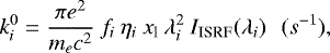 (A.1)
(A.1)
where f is the absorption oscillator strength that expresses the probability of absorption of electromagnetic radiation in transitions between energy levels of a molecule, η is the probability for dissociation of the upper level, xl is the fractional populations of the lower level and IISRF is the mean intensity of the ISRF in unit (photons cm−2 s−1 Å−1). The constant factor πe2∕mec2 takes the value 8.85 × 10⁻²¹ if λ is in Å. We have assumed xl has a Boltzmann distribution profile as follow:
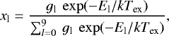 (A.2)
(A.2)
where gl and El are the degeneracy and energy of the lower level. Since in our model Tex (CO) = Tkin, to derive the fractional population of lower levels at the edge of the CSE, we considered Tex = 10 K which is the minimum acceptable temperature in our chemical network.
We considered the standard Draine radiation field Draine (1978) as the ISRF which has the form:
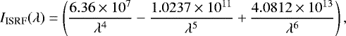 (A.3)
(A.3)
here I is in unit (ergs cm ). We multiplied I by a factor (5.03 × 10⁷ × λ) to convert the intensity unit to (photons cm−2 s−1 Å−1) which is needed in Eq. (A.1).
A.2 CO self-shielding
The CO self-shielding in an expanding spherical envelope was approximated by MJ83 to be:
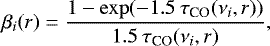 (A.4)
(A.4)
where βi(r) indicates the escape probability for a photon which is generated at radius r. When the absorption occurs primarily in the Doppler core of the line and by assuming that the CSE expansion velocity Vexp dominates the line width, the optical depth at the centre of each dissociating line νi can be written:
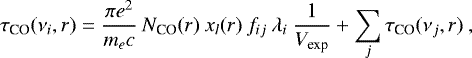 (A.5)
(A.5)
where NCO is a column density integrated from outside to r. The first term counts the CO optical depth at the centre of each dissociating line i and the second term counts the effect of all blended lines j if λi− λj < Δλj. Here, Δλj is the CO line broadening. In the first term πe2∕mec = 0.0265 and λ is in cm and Vexp is in cm s−1. The fractional population of the lower level xl varies by the radius here.
To derive τCO(νj, r) we have to estimate the line width of each dissociating line. Since the effect of the expansion velocity is equivalent for all lines, we need to onlyconsider the thermal and natural broadenings.
Thermal broadening
The thermal or Doppler broadening due to the random thermal motions of molecules has a gaussian profile as follows:
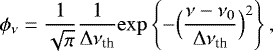 (A.6)
(A.6)
where the line of sight thermal width is defined as
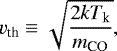 (A.7)
(A.7)
The peak value of ϕ(ν = ν0) is given by
 (A.9)
(A.9)
and the full-width at half maximum (FWHM):
 (A.10)
so the CO thermal broadening across the temperature range 10–2000 K is equivalent to 0.13–1.8 km s−1. These give the marginal line broadenings of Δλ1∕2 = (Δv1∕2∕c) λ ~ 0.4 × 10⁻³−0.6 × 10⁻² at the wavelength of 1000. Thus, we can ignore the thermal line broadening of CO.
Natural broadening
The natural line broadening resulting from the Heisenberg uncertainty principle gives a Lorentzian profile:
 (A.11)
where Γ is the quantum-mechanical damping constant and represents the total radiative decay probability or the inverse radiative lifetime of the upper level in s−1. The peak value of ϕ(ν = ν0) at the line centre is given by
 (A.12)
and the FWHM in frequency units will be:
 (A.13)
CO has Γ ~ 108−1013 s−1 which leads to the line broadening Δλ1∕2 = (λ2∕C)Δν1∕2 ~ (0.5 × 10⁻⁵−0.5). Thus, for the lines with large Γ the natural broadenings are significant.
As we now have the precise line positions and line widths of each individual line, we can estimate the number and contribution of blended lines in the opacity of each dissociating lines. We assumed that if λi − λj < Δλj, the j line is be considered in the second term of Eq. (A.5).
A.3 Mutual-shielding by H2 and dust
The shielding of CO by molecular hydrogen, H2, and dust in an expanding CSE is numerically approximated by MJ83 to be:
 (A.14)
where α = 1.644, b = 0.86.  is the H2 opacity at each CO dissociating line i and can be calculated as:
 (A.15)
here  is the H2 line shape at the CO line i. Since the H2 lines become optically thick, the absorption occurs in the radiative wings of the Lyman and Werner transitions. Thus, CO mutual-shielding by H2 mostly occurs at the Lorentzian damping wings of the H2 line profile (MJ83, MGH88) which is presented in Eq. (A.11). This gives the
H2 opacity at each CO dissociating line i:
 (A.16)
where m sums over all H2 dissociating lines.
In Eq. (A.14), we assumed that the dust absorption is independent of the wavelength in the spectral region of interest. We also ignored dust scattering and assume that the dust absorption dominates the dust extinction. Therefore, we considered a constant dust extinction at 1000, as MJ83, to be:
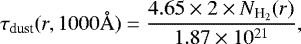 (A.17)
where  is the H2 column density to infinity.
Appendix B Grid models
Table B.1 presents the two fitting parameters of the CO envelope size for the full grid of models.
Fitting parameters α and r1∕2 which approximate the CO envelope size for all models.
References
- Abgrall, H., Roueff, E., Launay, F., & Roncin, J.-Y. 1994, Can. J. Phys., 72, 856 [NASA ADS] [CrossRef] [Google Scholar]
- Abgrall, H., Roueff, E., Liu, X., & Shemansky, D. E. 1997, ApJ, 481, 557 [NASA ADS] [CrossRef] [Google Scholar]
- Bally, J., & Langer, W. D. 1982, ApJ, 255, 143 [NASA ADS] [CrossRef] [Google Scholar]
- Danilovich, T., Bergman, P., Justtanont, K., et al. 2014, A&A, 569, A76 [NASA ADS] [CrossRef] [EDP Sciences] [Google Scholar]
- De Beck, E., Lombaert, R., Agúndez, M., et al. 2012, A&A, 539, A108 [NASA ADS] [CrossRef] [EDP Sciences] [Google Scholar]
- Draine, B. T. 1978, ApJS, 36, 595 [NASA ADS] [CrossRef] [Google Scholar]
- Garrod, R. T., & Herbst, E. 2006, A&A, 457, 927 [NASA ADS] [CrossRef] [EDP Sciences] [Google Scholar]
- Glassgold, A. E., Huggins, P. J., & Langer, W. D. 1985, ApJ, 290, 615 [NASA ADS] [CrossRef] [Google Scholar]
- Goldreich, P., & Scoville, N. 1976, ApJ, 205, 144 [NASA ADS] [CrossRef] [Google Scholar]
- Groenewegen, M. A. T. 2017, A&A, 606, A67 [NASA ADS] [CrossRef] [EDP Sciences] [Google Scholar]
- Habing, H. J., & Olofsson, H., eds. 2003, Asymptotic giant branch stars (Berlin: Springer Science & Business Media) [Google Scholar]
- Jura, M. 1974, ApJ, 191, 375 [NASA ADS] [CrossRef] [Google Scholar]
- Khouri, T., de Koter, A., Decin, L., et al. 2014, A&A, 561, A5 [NASA ADS] [CrossRef] [EDP Sciences] [Google Scholar]
- Lee, L. C. 1984, ApJ, 282, 172 [NASA ADS] [CrossRef] [Google Scholar]
- Letzelter, C., Eidelsberg, M., Rostas, F., Breton, J., & Thieblemont, B. 1987, Chem. Phys., 114, 273 [NASA ADS] [CrossRef] [Google Scholar]
- Li, X., Millar, T. J., Walsh, C., Heays, A. N., & van Dishoeck E. F. 2014, A&A, 568, A111 [NASA ADS] [CrossRef] [EDP Sciences] [Google Scholar]
- Maercker, M., Danilovich, T., Olofsson, H., et al. 2016, A&A, 591, A44 [Google Scholar]
- Mamon, G. A., Glassgold, A. E., & Huggins, P. J. 1988, ApJ, 328, 797 [NASA ADS] [CrossRef] [Google Scholar]
- McDonald, I., & Zijlstra, A. A. 2015, MNRAS, 446, 2226 [NASA ADS] [CrossRef] [Google Scholar]
- McDonald, I., Zijlstra, A. A., Lagadec, E., et al. 2015, MNRAS, 453, 4324 [NASA ADS] [CrossRef] [Google Scholar]
- McElroy, D., Walsh, C., Markwick, A. J., et al. 2013, A&A, 550, A36 [NASA ADS] [CrossRef] [EDP Sciences] [Google Scholar]
- Millar, T. J., Leung, C. M., & Herbst, E. 1987, A&A, 183, 109 [NASA ADS] [Google Scholar]
- Montez, Jr. R., Ramstedt, S., Kastner, J. H., Vlemmings, W., & Sanchez, E. 2017, ApJ, 841, 33 [NASA ADS] [CrossRef] [Google Scholar]
- Morata, O., & Herbst, E. 2008, MNRAS, 390, 1549 [NASA ADS] [Google Scholar]
- Morris, M., & Jura, M. 1983, ApJ, 264, 546 [NASA ADS] [CrossRef] [Google Scholar]
- Ramos-Medina, J., Sánchez Contreras, C., García-Lario, P., & da Silva Santos J. M. 2018, A&A, 618, A171 [NASA ADS] [CrossRef] [EDP Sciences] [Google Scholar]
- Ramstedt, S., & Olofsson, H. 2014, A&A, 566, A145 [NASA ADS] [CrossRef] [EDP Sciences] [Google Scholar]
- Ramstedt, S., Schöier, F. L., Olofsson, H., & Lundgren, A. A. 2008, A&A, 487, 645 [NASA ADS] [CrossRef] [EDP Sciences] [Google Scholar]
- Röllig, M., & Ossenkopf, V. 2013, A&A, 550, A56 [NASA ADS] [CrossRef] [EDP Sciences] [Google Scholar]
- Saberi, M., Maercker, M., De Beck, E., et al. 2017, A&A, 599, A63 [NASA ADS] [CrossRef] [EDP Sciences] [Google Scholar]
- Saberi, M., Vlemmings, W. H. T., De Beck, E., Montez, R., & Ramstedt, S. 2018, A&A, 612, L11 [NASA ADS] [CrossRef] [EDP Sciences] [Google Scholar]
- Scalo, J. M., & Slavsky, D. B. 1980, ApJ, 239, L73 [NASA ADS] [CrossRef] [Google Scholar]
- Schöier, F. L., & Olofsson, H. 2001, A&A, 368, 969 [NASA ADS] [CrossRef] [EDP Sciences] [Google Scholar]
- Solomon, P. M., & Klemperer, W. 1972, ApJ, 178, 389 [NASA ADS] [CrossRef] [Google Scholar]
- Van de Sande,M., & Millar, T. 2019, ApJ, 873, 36 [NASA ADS] [CrossRef] [Google Scholar]
- Van de Sande,M., Decin, L., Lombaert, R., et al. 2018, A&A, 609, A63 [NASA ADS] [CrossRef] [EDP Sciences] [Google Scholar]
- van Dishoeck, E. F., & Black, J. H. 1986, ApJS, 62, 109 [NASA ADS] [CrossRef] [Google Scholar]
- van Dishoeck, E. F., & Black, J. H. 1988, ApJ, 334, 771 [NASA ADS] [CrossRef] [Google Scholar]
- Visser, R., van Dishoeck, E. F., & Black, J. H. 2009, A&A, 503, 323 [NASA ADS] [CrossRef] [EDP Sciences] [Google Scholar]
All Tables
Comparison of the fitting parameters of the CO envelope between this work and MGH88.
Fitting parameters α and r1∕2 which approximate the CO envelope size for all models.
All Figures
|
Fig. 1 CO fractional abundance distributions for simulations with different shielding functions that regulate CO photodissociation: shielding by H2, shielding by dust, CO self-shielding, and the total shielding for the reference model. |
| In the text | |
|
Fig. 2 CO fractional abundance distributions for models with a constant expansion velocity Vexp = 15 (km s−1) and various Ṁ (M⊙ yr−1) and fCO in a way to keep the same amount of effective CO for all models. |
| In the text | |
|
Fig. 3 CO fractional abundance distributions for models with fCO = 8 × 10⁻⁴, Vexp = 15 (km s−1), and a range of mass-loss rates which are marked in the figure. |
| In the text | |
|
Fig. 4 Comparison of the CO fractional abundance distributions from modelling (solid black lines) and the analytic fitting formula (dashed blue lines) for models with fCO = 8 × 10⁻⁴, Vexp = 15 (km s−1) and a range of 10−8 < Ṁ < 10−4 (M⊙ yr−1). |
| In the text | |
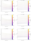 |
Fig. 5 Variation of two fitting parameters α and r1∕2 for all models presented in Table B.1. |
| In the text | |
|
Fig. 6 Left panel: tested gas kinetic temperature profiles with different β values. Theprofile with label “reference” corresponds to the temperature of the reference model. Right panel: CO abundance distribution profile derived using the temperature profiles from the left panel. |
| In the text | |
|
Fig. 7 CO fractional abundances distributions for the reference model when different CO excitation temperature profiles are considered in calculations of the CO photodissociation rate. |
| In the text | |
|
Fig. 8 Comparison of CO abundance distribution parameters to MGH88 results. The left panel shows
|
| In the text | |
|
Fig. 9 Results of CO RT modelling for model 1 (the reference model) with the CO abundance distribution from this work (red) and MGH88 (blue). The transitions and the beam size are marked in each panel. Bottom right panel: compares the radial distribution of the CO(1–0) integrated intensities at radial offset points. |
| In the text | |
|
Fig. 10 Results of CO RT modelling for model 2 with extreme discrepancy between the CO abundance distribution from this work (red) and MGH88 (blue). The transitions and the beam size are marked in each panel. The bottom right panel compares the radial distribution of the CO(1–0) integrated intensities at radial offset points. |
| In the text | |
Current usage metrics show cumulative count of Article Views (full-text article views including HTML views, PDF and ePub downloads, according to the available data) and Abstracts Views on Vision4Press platform.
Data correspond to usage on the plateform after 2015. The current usage metrics is available 48-96 hours after online publication and is updated daily on week days.
Initial download of the metrics may take a while.