| Issue |
A&A
Volume 624, April 2019
|
|
|---|---|---|
| Article Number | A45 | |
| Number of page(s) | 10 | |
| Section | Planets and planetary systems | |
| DOI | https://doi.org/10.1051/0004-6361/201834592 | |
| Published online | 04 April 2019 | |
New metric to quantify the similarity between planetary systems: application to dimensionality reduction using T-SNE★
Physikalisches Institut & NCCR PlanetS, Universität Bern, 3012 Bern, Switzerland
e-mail: alibert@space.unibe.ch
Received:
7
November
2018
Accepted:
24
January
2019
Context. Planet formation models now often consider the formation of planetary systems with more than one planet per system. This raises the question of how to represent planetary systems in a convenient way (e.g. for visualisation purpose) and how to define the similarity between two planetary systems, for example to compare models and observations.
Aims. We define a new metric to infer the similarity between two planetary systems, based on the properties of planets that belong to these systems. We then compare the similarity of planetary systems with the similarity of protoplanetary discs in which they form.
Methods. We first define a new metric based on mixture of Gaussians, and then use this metric to apply a dimensionality reduction technique in order to represent planetary systems (which should be represented in a high-dimensional space) in a two-dimensional space. This allows us study the structure of a population of planetary systems and its relation with the characteristics of protoplanetary discs in which planetary systems form.
Results. We show that the new metric can help to find the underlying structure of populations of planetary systems. In addition, the similarity between planetary systems, as defined in this paper, is correlated with the similarity between the protoplanetary discs in which these systems form. We finally compare the distribution of inter-system distances for a set of observed exoplanets with the distributions obtained from two models: a population synthesis model and a model where planetary systems are constructed by randomly picking synthetic planets. The observed distribution is shown to be closer to the one derived from the population synthesis model than from the random systems.
Conclusions. The new metric can be used in a variety of unsupervised machine learning techniques, such as dimensionality reduction and clustering, to understand the results of simulations and compare them with the properties of observed planetary systems.
Key words: planets and satellites: formation / methods: data analysis / methods: numerical / methods: statistical
The movie associated to Fig. 11 is available at https://www.aanda.org
© ESO 2019
1 Introduction
Since the discovery of the first exoplanet orbiting a solar-type star (Mayor & Queloz 1995), numerous planets have been discovered, a non-negligible fraction of them being part of planetary systems with more than one planet. One recent example is the discovery of the Trappist-1 system harbouring seven planets with known mass, radius, orbital elements, and composition (e.g. Gillon 2017; Grimm et al. 2018; Dorn et al. 2018). At the same time, different groups have developed theoretical and numerical models with the aim of computing the properties of planetary systems (Ida & Lin 2004, 2010; Alibert et al. 2013, Emsenhuber et al., in prep.). One goal of these models is to improve our knowledge of the physical processes at work during planet formation by comparing theoretical results with observations.
These comparisons have in general focussed on the properties of planets (e.g. mass distribution, radius distribution, mass-radius correlation), but not on the global properties of planetary systems1. The dimensionality of a planetary system (the number of quantities that characterise it) scales with the number of planets in the system, and can be quite large. If we only consider mass and semi-major axis, for example, we need 2N parameters to characterise a system with N planets. Comparing sets of data (e.g. results of simulations on one side, observations on the other side) is not easy as soon as the number of planets is larger than 1, and the purpose of the present paper is to propose a metric (or distance) in the space of planetary systems for quantitatively comparing different planetary systems. This distance can be used to discover classes of systems in simulations or observations. We note that throughout this paper the word “distance” is used to designate the mathematical distance between two planetary systems in a high-dimensional space, and is not related with any physical distance (e.g. semi-major axis, physical distance between the observer and a star). In the same way, we then introduce the concept of density of a planetary system, which is not related in any way to the physical bulk density of a planet.
The paper is organised as follows. In Sect. 2 we introduce the distance between planetary systems. In Sect. 3 we then use this distance to represent planetary systems (which belong intrinsically to a high-dimensional space) in a 2D space, using a dimensionality reduction technique named T-SNE. We use the same technique to relate the similarity between planetary systems with the similarity of protoplanetary discs in which they form. Finally, we discuss our results, in particular possible improvements of the distance we propose, in Sect. 4.
2 Constructing a distance in the space of planetary systems
2.1 Properties of distances
We start by recalling the properties of a distance. A distance on a space S is a function d from S2 to  with the following properties:
-
d(x, y) = 0 ⇔ x = y,
-
d(x, y) = d(y, x),
-
d(x, y) ≤ d(x, z) + d(z, y) for every x,y,z in S.
A function d which fulfils only the first two properties but not the last one (the triangular inequality) is called a pseudo-distance. It is important to remember that many machine learning techniques and algorithms require the use of a distance and fail when using a pseudo-distance (Bishop 2006; Goodfellow et al. 2016). For this reason it is important that the distance between planetary systems that we construct respects the triangular inequality.
In the special case of comparing planetary systems with only one planet, an easy and natural way is to directly compute the Euclidian distance between the two points representing the planets in the feature space (e.g. mass and semi-major axis). For example, we can define the distance between system s1 and system s2 as
 (1)
(1)
where M1, M2 and a1, a2 are the masses and semi-major axes of the planet in system 1 and system 2, respectively, expressed in a relevant unit. We note that we could also use directly M and a (and not their logarithms) to define the distance. Given the very wide range of values these parameters can take, however, this would be impractical. This distance is the Euclidian distance, so it fulfils the three above-mentioned properties.
This definition gives the same importance to both the mass and semi-major axis. However, this can be changed by adding some positive constant factors αM and αa to obtain
 (2)
(2)
For the rest of the paper, we assume that planets are characterised by only two features: the logarithm of the mass M and of the semi-major axis a. The generalisation to the case where more features characterise the planets (e.g. the radius, composition) is straightforward.
2.2 Density distance
When more than one planet exists in each system, and assuming for the time that both systems harbour the same number of planets, we intuitively judge the similarity between the two systems by looking at the distance each planet from s1 is from another planet from s2. Still intuitively, we would like to define thedistance between s1 and s2 as the sum (or the maximum) of the distances between the pairs planets (one belonging to s1, the other belonging tos2). However, this approach suffers from the problem that there are many ways to construct the pairs of planets and the resulting distance between the two systems may depend on the choice of these pairs. One way to avoid this arbitrariness is to rank the planets in each system (for example by mass) and to compare the lower mass planet in s1 with the lower mass planet in s2 and so on. However, this sill leads to some unwanted behaviour, as shown in Fig. 1. In the left panel we compare two systems, and the ranking by mass leads to the comparison between the planets indicated by the arrows. The distance between these two systems is small. In the right panel, the system depicted in blue has been modified, the most massive planet being now the innermost one (and not the outermost one, as in the left panel). In this case, the distance between the two systems is computed comparing the planets indicated by the arrows, and the resulting distance is much larger than in the left panel. This is not satisfactory since we intuitively would like to consider that the two situations are very similar, so the inter-system distances in both cases should be very close.
One way to avoid the problem of choosing pairs is to use the Hausdorff distance (Hausdorff 1914):
 (3)
(3)
The Hausdorff distance by definition fulfils the three properties of mathematical distances, but it gives the same importance to all planets in the system (see next section).
Another way to construct the distance between systems, and also avoid the problem of choosing pairs of planets, is to first define the density of a system. To this end, we first define for each planet p in a system s a function fp (M, a) given by
 (4)
(4)
where Mp and ap are the mass and semi-major axis of the planet, and σM and σa are constants, taken as equal to 1∕0.3 for the rest of the paper (we discuss below and in Sect. 4 the influence of these values). The function fp (M, a) “smears out” the planet p and the constants σM and σa giving the scale of this smearing out in the log M and log a directions. We can finally define the density ψs of a system s as
 (5)
(5)
Figure 2 gives an example of the density ψ of a system with three planets. The red rectangle covers a range in log a extending from −2 to +2 (0.01–100 AU since a is expressed in AU), and a range in log M extending from −2 to +4 (0.01 M⊕ –104M⊕).
Finally, the distance between two systems s1 and s2 is given by
 (6)
(6)
The integral should be extended to infinity, but in practical cases it is sufficient to extend the integral to a large enough domain. In the examples that follow, we integrate over a domain ranging from −10 to 10 both in log M and log a.
The choice of the parameters αM and αa has some arbitrariness, and can be used to vary the importance of the mass and the semi-major axis in the determination of the distance. A small value of the parameter corresponds to a reduced importance of the corresponding quantity in the computation of the distance. In the limiting case of a value equal to 0, the corresponding parameter does not enter in the computation of the distance. Since these parameters correspond to the scale on which the planets are smeared out, a natural choice could be to use the observational uncertainties (in the case some observations are considered).
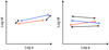 |
Fig. 1 Examples of computation of distance between two planetary systems. See text for details. |
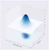 |
Fig. 2 Density of a planetary system ψ with three planets (100 M⊕ at 0.02 AU, 10 M⊕ at 1 AU, 0.02 M⊕ at ~ 80 AU, represented as red points). The σM and σa parameters are both equal to 1∕0.3. |
2.3 Weighted distance
One problem with the distances presented in the previous section is that all planets in a system have the same importance. The functions fp all have the same integral, so a super-Jupiter and a sub-moon contribute in a similar way to the distance between two systems. One consequence is that the distance between a system s1 and a system s2 that is similar but contains in addition a tiny planet is non-zero. In order to mitigate this effect, we introduce in the definition of the functions fp a weight that depends on the properties of the planet. Here again, the choice of the weighting is arbitrary, but must be the same for all systems. One possibility is to have a weight proportional to the logarithm of the mass of the planet, or proportional to the inverse of the period of the planet (planets located far from their star contributing less) or to its radial velocity semi-amplitude if the aim is to compare systems that are observed by radial velocity. In what follows we choose to weight the function proportionally to the logarithm of the mass of the planet, independently of the period. In addition, the integral of the Ψ function for each system is proportional to the logarithm of the total mass in the system.
2.4 Distance distribution in a population of synthetic planetary systems
The population of systems that we use to illustrate the use of the distance presented in this paper have been computed using an updated version of the code of Alibert et al. (2005, 2013), Mordasini et al. (2009a,b, 2012a,b, 2015), and Fortier et al. (2013). In this model, we follow the growth and orbital evolution of ten planetary embryos in a protoplanetary disc, taking into account growth by gas and solid accretion, orbital evolution by disc-planet interactions, and planet–planet interactions. We do not take into account in these models enrichment of planetary envelopes by heavy elements (Venturini et al. 2015, 2016; Venturini & Helled 2017). The gas surface density in the initial protoplanetary disc is given by
![\begin{equation*} \Sigma = (2 - \gamma) { M_{\textrm{disc}} \over 2 \pi a_C^{2-\gamma} r_0^{\gamma} } \left( {r \over r_0} \right)^{\gamma} \exp \left[ - \left( {r \over a_C}^{2-\gamma} \right) \right], \end{equation*}](/articles/aa/full_html/2019/04/aa34592-18/aa34592-18-eq8.png) (7)
(7)
where r0 is equal to 5.2 AU, and Mdisc, aC, and γ are derived form the observations of Andrews et al. (2010). This gas surface density evolves as a result of viscous transport (in the framework of the α viscosity model) and photoevaporation (see references above for details of the numerical model). As in Mordasini et al. (2009a), the planetesimal-to-gas ratio is assumed to scale with the metallicity of the central star. For every protoplanetary disc we consider, we therefore select at random the metallicity of a star from a list of ~ 1000 CORALIE targets (Santos, priv. comm.). Finally, following Mamajek (2009), we assume that the cumulative distribution of disc lifetimes decays exponentially with a characteristic time of 2.5 Myr. When a lifetime Tdisc is selected (at random, following the above-mentioned cumulative distribution), we adjust the photoevaporation rate such that the protoplanetary disc mass reaches 10−5M⊙ at the time t = Tdisc, and then westop the calculation. After the disc dispersal, the system is further evolved for some time (computing planet–planet interactions and cooling of planets), the total simulated time for formation and evolution being 20 Myr. In each of these discs, ten planetary embryos are present at the beginning of the simulation. The initial location of the embryos is chosen at random, following a distribution uniform in logarithm. The updated code is presented in Emsenhuber et al. (in prep.), but we note that the focus of the present paper is to propose a new metric. Application to the most recent simulations (with 50 or 100 planetary embryos growing in the same protoplanetary disc) will be presented in a future paper.
The population we use is shown in Fig. 3, upper panel, where all planets belonging to the same planetary system are linked by a straight line. A planetary system is then represented as a broken line with up to nine changes of slope since it can contain up to ten planets at the end of the simulation (some may be ejected, may collide with other planets, or may be engulfed in the central star).
In order to compare the distribution of inter-system distances with that of another population, we constructed a set of non-physical systems in the following way. We took all the planets in our reference population and produced new systems by drawing at random without replacement up to ten planets. The distribution of the number of planets per system in these non-physical systems is the same as for the reference population. We show in Fig. 3, lower panel, these non-physical planetary systems, where it can be seen from the geometry of the broken lines that there are systematic differences between the two populations. We note that we have not added any constraint during the construction of the non-physical population, meaning that some of them could well be dynamically unstable or impossible to form.
The distribution of the distances in the two populations is shown in Fig. 4, where it is clear that the non-physical systems are more similar to each other (the distribution of distances, in red in the figure, is narrower). This is not surprising, since by shuffling planets between systems of the reference population, we have destroyed any correlation between planets in the same system, which could lead to systems being less similar to each other. This demonstrates, as was expected, that a system of ten planets produced by the numerical simulation is not just a collection of ten independent planets.
The reference population shows two peaks, for distances of around 0.1 and 0.4. In Figs. 5 and 6 we show pairs of systems with mutual distances equal to 0.4 and 0.1. As can be seen in Fig. 5, pairs of systems with a mutual distance close to 0.4 (the second peak in the distance distribution) are generally very dissimilar: one system harbours massive planets (in particular at an intermediate semi-major axis), one system only harbours low-mass planets. Moreover, the systems with massive planets (represented in blue) in general harbour fewer planets. The structure of the systems with small planets (represented in red) is generally regular, and such systems are very unlikely to exist in the non-physical population. This explains the absence of a peak at a similar large distance in the histogram shown in Fig. 4 for the non-physical population. On the contrary, pairs of systems with mutual distance close to 0.1 shown in Fig. 6 are in general either both with low-mass planets or both with larger planets. In addition, they have similar numbers of planets; some of them are less regular than the ones shown in Fig. 5.
Although the populations used in this paper have not been computed with the most recent code (with up to 50 or 100planetary embryos growing in the same protoplanetary disc; see Emsenhuber et al., in prep.) we have compared in Fig. 7 the cumulative distance distribution of both the reference and the non-physical populations with a population of actual exoplanets planets detected (the “RV” population). To this end, we have selected planetary systems (with more than one planet) orbiting around stars of mass between 0.85 M⊙ and 1.15 M⊙ (assuming a solar-type central star). Since we use in this paper the mass and semi-major axis as primary planet parameters, we have only taken into accountsystems for which the masses of all known planets has been measured. We have then, for both synthetic populations (the reference and the non-physical), retained only planets whose period is less than 5 yr, and radial velocity semi-amplitude is larger than 3 m s−1. These values were chosen in order to approximately match the range of parameters of the observed planets (RV population) we have considered2. The cumulative distribution of the RV population is closer to that of the reference population than to that of the non-physical population, even though the match between the RV and the reference populations is not perfect.
We finally note that the distributions of the two simulated populations are much closer to each other than to the cumulative distributions corresponding to Fig. 4. This results from considering only planets with small period and large radial velocity semi-amplitude.
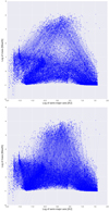 |
Fig. 3 Reference population (upper panel) and non-physical population (bottom panel). In each panel, planets are represented by points in the log a– log M space (whereM is in M⊕ and a is in AU). Planets belonging to the same system are linked by a line; a planetary system is therefore represent by a broken line with up to nine changes of slope. |
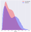 |
Fig. 4 Distribution of the inter-system distances in the reference population (blue) and the non-physical population (red). |
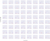 |
Fig. 5 Examples of pairs of systems with mutual distance close to 0.4 (second peak in the distance distribution of Fig. 4) for the reference population. In each sub-panel, the system represented in red is the one with the lowest maximum mass. The axis in each panel has been omitted for clarity; the range for each axis is the same as in Fig. 3. |
3 Systems representation using low-dimensional embedding
3.1 T-SNE
The distance we propose in the present paper can be used in the framework of unsupervised machine learning, for example for dimensionality reduction. As already pointed out in the introduction, representing a planetary system with N planets, each of them being characterised by two quantities, requires a space of dimension 2N. The goal of dimensionality reduction algorithms is to represent the planetary systems in a space of dimension 2 (or 3) while keeping as much information as possible regarding their repartition in the space of dimension 2N.
Different dimensionality reduction algorithms have been developed; we use here T-SNE (for t-based stochastic neighbour embedding, see van der Maaten & Hinton 2008) to represent systems of up to ten planets in a 2D space. The T-SNE algorithm (van der Maaten 2014) works in two steps. In a first step, the joint probability of two systems is computed. The joint probability between systems i and j depends on the distance between two systems (computed using the distance presented above) as
 (8)
(8)
where σ is a parameter called the perplexity that controls the number of neighbours (see van der Maaten 2014). Then, an iterative algorithm is used to minimise a cost function given by the Kullback–Leibler divergence (Kullback & Leibler 1951) of the p distribution and the q distribution, where q is the joint probability of two systems in the 2D space, function of the distance between the points representing systems i and j in the 2D space, and assumed to follow a Student’s t-distribution with one degree of freedom (also known as the Cauchy or Lorentz distribution)
 (9)
(9)
where ||.|| is the Euclidian norm in the 2D space. The Kullback–Leibler divergence from q to p (also called relative entropy) is given by
 (10)
(10)
where S is the population of systems being considered. This function measures the loss of information occurring when using the q distribution instead of the p distribution. If two points are similar (large pi,j or small distance) in the 2N dimension space, they have tobe close in the 2D space in order to avoid a large cost. If, on the other hand, two points are very dissimilar (large distance in the 20 dimension space), there are no real constraints as the contribution to the cost function is small, whatever the value of qi,j.
An important point of the T-SNE algorithm is that the cost function is not convex; in particular, it is invariant by translation and rotation in the 2D space. As a consequence, the result of T-SNE is not unique and it is advised to run the algorithm a number of times, slightly changing the initial position of the systems in the 2D space in order to distinguish features that are robust from spurious structures.
The result of the T-SNE visualisation for the two populations we consider is shown in Fig. 8, where the colour-coding indicates the number of planets at the end of the simulation. It is important to emphasise that a planetary system is represented in this diagram by a single point; instead, in Fig. 3 a planetary system is represented by a broken line with up to nine changes of slope. In addition, the number of planets is not an input of the T-SNE algorithm which only uses the mutual distance between systems. Finally, it is important to note that the T-SNE components of the systems have no physical meaning and cannot be related to the physical properties of the systems or the planets belonging to them.
In the upper panel, in the case of the reference population, a non-random distribution is seen where systems with the same (or nearly the same) number of planets lie close together. This means that these systems are also close (or similar) in the 20 dimension space. On the contrary, systems with only one planet lie far from all systems with 10 planets and they are therefore very different. This can be confirmed by examining these two classes of systems (10 planets versus 1 planet) in the log a– log M space (see Fig. 9). As can be seen in this figure, systems with only one planet have a very different architecture (massive planet, located in general far from the central star) compared to ten-planet systems (in general low-mass planets with a wide range of semi-major axes).
Another interesting feature is that systems with ten planets (light green points) are not clustered in the same part of the diagram. Comparing the ten-planet systems in the left part of the diagram (in the red rectangle) and in the right part (in the blue rectangle), in the log a– log M space (see Fig. 10) we see that these two classes correspond to systems with only low-mass planets or only more massive planets, respectively. These two classes are very well separated, planets represented in red and in blue lying on opposite sides of a part of the log a– log M diagram where very few planets exist3. Finally, the systems depicted in blue in Fig. 10 (in the blue rectangle in Fig. 8) are located closer to systems with only one planet on the T-SNE representation (Fig. 8). This is to be expected since the planets in these systems are more massive, and more similar to the planets in the one-planet systems (Fig. 9).
In the case of the non-physical population (lower panel of Fig, 8), the distribution is very different with little spatial segregation between systems with a different number of planets. This again shows that there is a structure in the reference population that is lost when constructing the non-physical systems.
 |
Fig. 6 Same as Fig. 5, but for pairs of systems whose mutual distance is close to 0.1 (first peak in the distance distribution of Fig. 4). |
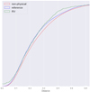 |
Fig. 7 Cumulative normalised distributions of the mutual distances for the reference, the non-physical, and the RV populations. Only planets with a period less than 5 yr and radial velocity semi-amplitude larger than 3 m s−1, and (for the RV population) orbiting around stars of mass between 0.85 M⊙ and 1.15 M⊙ have been considered. |
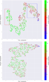 |
Fig. 8 T-SNE visualisation of the reference population (upper panel) and the non-physical population (lower panel). The colour-coding indicates the number of planets that remain at the end of the planetary system formation model. The blue and red rectangles indicate two sub-classes of systems whose properties are compared in Figs. 9 and 10; see text for details. |
3.2 Link with protoplanetary disc properties
An important question is whether the similarity between planetary systems is linked to the similarity of the protoplanetary discs in which they form. In order to answer this question, we need first to define the similarity between discs in the space of disc parameters. In our simulations, each disc model depends on five parameters, Σgas, Σsolids, aC, γ, photoevaporation rate, where Σgas and Σsolids are respectively the values of the gas surface density at 5.2 AU and the product of this surface density and the dust-to-gas ratio. These two parameters are equivalent to the total disc mass and the dust-to-gas ratio. Using these five parameters, we can easily define a metric in the space of disc parameters by using the Euclidian distance in this 5D space. In order to avoid differences that are too large between the scales of the different parameters, we use the logarithm of the disc parameters, and scale them to obtain the same mean and variance for all these quantities. This is arbitrary since it gives all the parameters the same importance in the determination of the metric, but since it is not clear which disc parameter is most important, it is a natural and conservative choice.
Using this new metric, we can run T-SNE to compute a 2D embedding of the disc models (which originally belong to a 5D space), and infer wether the embedding can be related to that computed using the metric in the planetary system space. For this, we first assign a colour to each of the points in Fig. 8, which is related to its position in the figure (see Fig. 11, upper panel). Then, we plot in Fig. 11, lower panel, the T-SNE embedding (computed using the disc parameter metric), using the same colours. As can be seen in the figure4, the colour gradient in the upper panel is largely preserved in the lower panel. For example, light green-blue points (which correspond to ten-planet systems with low masses) in the upper panel are preferentially located in the lower left region of the lower panel. The discs in which these low-mass ten-planet systems form are therefore similar (in terms of the disc parameter metric). However, the colour gradient is not totally preserved as some local variations in the colours can be seen. This shows that other parameters (e.g. the initial location of the planetary embryos) are also important in governing the final architecture of planetary systems.
This finding is confirmed in Fig. 12, where we show the relation between the inter planetary system distance (using the metric introduced in Sect. 2.3), and the distance between the same systems computed using the disc parameters. The correlation between the two distances is clear, with some notable dispersion that is due to the other initial conditions of the formation calculations, such as the starting location of the planetary embryos.
In conclusion, the disc parameters govern the trend in the planetary system architecture, while some special circumstances (e.g. special starting locations of planetary embryos) can lead to local variations.
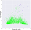 |
Fig. 9 Systems in the reference population with ten planets (green) and one planet (blue). |
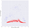 |
Fig. 10 Systems in the reference population with ten planets whose T-SNE representation lie in the red and blue rectangles in the upperpanel of Fig. 8. The large grey dots are systems with only one planet, which are more similar to the systems represented in blue than to the one represented in red. |
4 Discussion and conclusion
We have presented in this paper a new metric to compare planetary systems, and have illustrated it with two synthetic populations of planets. The distance we have defined has two free parameters in the definition of the Ψ functions (parameters σM and σa). The value to be chosen for these two parameters is not very important as the correlation between two sets of distances (computed using two set of parameters) is very strong (see Fig. 13). It is important to note that it is the ranking of the distances between the systems that is important (which system is at a greater distance than another from a reference system) and not the absolute value of the distance between two systems. We also note that the study presented in this paper relates vectors representing planetary systems on the one hand, and protoplanetary discs on the other. Whether these vectors are accurate representations of real planetary systems and protoplanetary discs remains to be established.
Using the distance in the space of planetary systems, we have shown that population synthesis models produce a structure in the architecture of planetary systems that is intrinsically different from what would be obtained by just randomly drawing a set of up to ten planets taken from the global population of planets. In addition, we have shown that the similarity between systems is related to the similarity between the protoplanetary discs in which they form. We have not studied the population of systems beyond these two cases since the population we used as an example here will be updated in a future paper (Emsenhuber et al., in prep.). The detailed study of the architecture of systems using the methods presented here will be the subject of a forthcoming paper (Alibert et al., in prep.).
The metric we have presented in this paper encapsulates the comparison between masses and semi-major axes of all planets in different systems. It can be easily extended to the case where several properties are known for each planet (e.g. the radius) in a straightforward way. We note, however, that as the number of features increases, the number of data points needed to analyse the results of simulations or observations grows exponentially and can rapidly become untraceable. This is an effect of the well-known “curse of dimensionality” (e.g. Goodfellow et al. 2016).
Some aspects of the architecture of planetary systems are not included in this metric. For example, this is the case for the presence of resonances (e.g. mean motion resonances) in systems. Indeed, a slight variation in the semi-major axis of one planet in a system does not modify strongly the Ψ function of this system. As a consequence, two systems can be very similar (according to the metric we propose in the present paper) even though one could be in mean motion resonance and the other out of resonance. Taking into account the resonant configurations of planetary systems requires modifications of the metric, in essence by adding an extra dimension to the system. This will be explored in a future paper (Alibert et al., in prep.).
We finally note that we have weighted the contribution of planets in the determination of the Ψ function using the logarithm of the mass. This is arbitrary and may not be the optimal choice. Such a choice indeed means that the mass of a small planet in a system is not very important. On the other hand, in the precise case of the solar system, the fact that Mars has a low mass is one of the foundations of our present understanding of the formation of the solar system (see Walsh et al. 2011 in the framework of the Grand Tack model). In this case, it would be legitimate to believe that our solar system, and the same system where Mars would have a mass similar to that of the Earth could be fundamentally different (at least in terms of theformation process). However, in the case of exoplanets, the level of detail of the present observational constraints is far from the level of detail we have for the solar system, and the metric presented here, although it will certainly have to be improved in the future, gives a useful framework for comparing the global trends of models and observations.
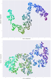 |
Fig. 11 T-SNE representation based on the distance in the space of systems (upper panel) and distance in the space of disc parameters (lower panel). The upper panel is similar to Fig. 8, upper panel, except that here the colour-coding is only linked to the position of the point on the plot. In the lower panel, we used T-SNE based on the similarity resulting from the metric in the space of disc parameters (see text) to represent systems. The colour-coding indicates in which part of the upper panel the same system is represented. In the lower panel, two points located close to each other represent planetary systems formed in similar discs, whereas two points with similar colours represent planetary systems that are themselves similar. An animation is available online. |
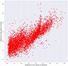 |
Fig. 12 Correlation between the inter systems distance (horizontal axis) and the distance computed using the disc parameters (vertical axis) for a sub-set of 5000 points. |
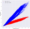 |
Fig. 13 Effect of changing the parameters in the computation of the Ψ function. Here, 5000 inter-system distances are computed for σM = σa = 1 (red) and σM = σa = 1∕10 (blue) and compared with the distance using reference values for the same systems. The correlation between the reference and the newdistance is clearly seen. |
Movie
Movie of Fig. 11 Access here
Acknowledgements
We thank Julia Venturini for the enlightening discussions. This work has been carried out within the frame of theNational Centre for Competence in Research PlanetS supported by the Swiss National Science Foundation. The author acknowledges the financial support of the SNSF.
References
- Alibert, Y., Mordasini, C., Benz, W., & Winisdoerffer, C. 2005, A&A, 434, 343 [NASA ADS] [CrossRef] [EDP Sciences] [Google Scholar]
- Alibert, Y., Carron, F., Fortier, A., et al. 2013, A&A, 558, A109 [NASA ADS] [CrossRef] [EDP Sciences] [Google Scholar]
- Andrews, S. M., Wilner, D. J., Hughes, A. M., Qi, C., & Dullemond, C. P. 2010, ApJ, 723, 1241 [NASA ADS] [CrossRef] [Google Scholar]
- Bishop, C. M. 2006, Pattern Recognition and Machine Learning (Berlin: Springer) [Google Scholar]
- Dorn, C., Mosegaard, K., Grimm, S., & Alibert, Y., 2018, ApJ, 865, 20 [NASA ADS] [CrossRef] [Google Scholar]
- Fortier, A., Alibert, Y., Carron, F., Benz, W., & Dittkrist, K. M. 2013, A&A, 549, A44 [NASA ADS] [CrossRef] [EDP Sciences] [Google Scholar]
- Gillon, M., Triaud, A. H. M. J., Demory, B.-O., et al., 2017, Nature, 542, 456 [NASA ADS] [CrossRef] [PubMed] [Google Scholar]
- Goodfellow, I., Bengio, Y., & Courville, A., 2016, Deep Learning (Cambridge: MIT press) [Google Scholar]
- Grimm, S. L., Demory, B.-O., Gillon, M., et al. 2018, A&A, 613, A68 [NASA ADS] [CrossRef] [EDP Sciences] [Google Scholar]
- Hausdorff, F. 1914, Grundzüge der Mengenlehre (Leipzig: Veit) [Google Scholar]
- Ida, S., & Lin,D. 2004, ApJ, 616, 567 [NASA ADS] [CrossRef] [MathSciNet] [Google Scholar]
- Ida, S., & Lin,D. 2010, ApJ, 719, 810 [NASA ADS] [CrossRef] [Google Scholar]
- Kullback, S., & Leibler, R. A. 1951, Ann. Math. Stat., 22, 79 [CrossRef] [Google Scholar]
- Mamajek, E. E. 2009, AIP Conf. Ser., 1158, 3 [Google Scholar]
- Mayor, M., & Queloz, D. 1995, Nature, 378, 355 [NASA ADS] [CrossRef] [Google Scholar]
- Mordasini, C., Alibert, Y., & Benz, W. 2009a, A&A, 501, 1139 [NASA ADS] [CrossRef] [EDP Sciences] [Google Scholar]
- Mordasini, C., Alibert, Y., & Benz, W. 2009b, A&A, 596, 90 [Google Scholar]
- Mordasini, C., Alibert, Y., Klahr, H., & Henning, T. 2012a, A&A, 547, A111 [NASA ADS] [CrossRef] [EDP Sciences] [Google Scholar]
- Mordasini, C., Alibert, Y., Georgy, C., et al. 2012b, A&A, 547, A112 [NASA ADS] [CrossRef] [EDP Sciences] [Google Scholar]
- Mordasini, C., Molliere, P., Dittkrist, K.-M., Jine, S., & Alibert, Y. 2015, IJASB, 14, 201 [NASA ADS] [Google Scholar]
- Pfyffer, S., Alibert, Y., Benz, W., & Swoboda, D. 2015, A&A, 579, A37 [NASA ADS] [CrossRef] [EDP Sciences] [Google Scholar]
- van der Maaten, L. J. P. 2014, J. Mach. Learn. Res., 15, 3221 [Google Scholar]
- van der Maaten, L. J. P., & Hinton, G. E. 2008, J. Mach. Learn. Res., 9, 2579 [Google Scholar]
- Venturini, J., & Helled, R. 2017, ApJ, 848, 95 [NASA ADS] [CrossRef] [Google Scholar]
- Venturini, J., Alibert, Y., Benz, W., & Ikoma, M. 2015, A&A, 576, A114 [NASA ADS] [CrossRef] [EDP Sciences] [Google Scholar]
- Venturini, J., Alibert, Y., & Benz, W. 2016, A&A, 576, A114 [Google Scholar]
- Walsh, K. J., Morbidelli, A., Raymond, S. N., O’Brien, D. P., & Mandell, A. M. 2011, Nature, 475, 7355 [Google Scholar]
One exception is the study of the distribution of period ratios in planetary systems; see e.g. Pfyffer et al. (2015).
The presence of this region with very few planets results because we have not considered ten-planet systems outside the blue and red rectangles, as can be seen from Fig. 9, which shows in light green all the planets belonging to ten-planet systems.
An animation showing the transition from the first to the second representation can be found online and at http://nccr-planets.ch/research/phase2/domain2/project5/machine-learning-and-advanced-statistical-analysis/
All Figures
|
Fig. 1 Examples of computation of distance between two planetary systems. See text for details. |
| In the text | |
|
Fig. 2 Density of a planetary system ψ with three planets (100 M⊕ at 0.02 AU, 10 M⊕ at 1 AU, 0.02 M⊕ at ~ 80 AU, represented as red points). The σM and σa parameters are both equal to 1∕0.3. |
| In the text | |
|
Fig. 3 Reference population (upper panel) and non-physical population (bottom panel). In each panel, planets are represented by points in the log a– log M space (whereM is in M⊕ and a is in AU). Planets belonging to the same system are linked by a line; a planetary system is therefore represent by a broken line with up to nine changes of slope. |
| In the text | |
|
Fig. 4 Distribution of the inter-system distances in the reference population (blue) and the non-physical population (red). |
| In the text | |
|
Fig. 5 Examples of pairs of systems with mutual distance close to 0.4 (second peak in the distance distribution of Fig. 4) for the reference population. In each sub-panel, the system represented in red is the one with the lowest maximum mass. The axis in each panel has been omitted for clarity; the range for each axis is the same as in Fig. 3. |
| In the text | |
|
Fig. 6 Same as Fig. 5, but for pairs of systems whose mutual distance is close to 0.1 (first peak in the distance distribution of Fig. 4). |
| In the text | |
|
Fig. 7 Cumulative normalised distributions of the mutual distances for the reference, the non-physical, and the RV populations. Only planets with a period less than 5 yr and radial velocity semi-amplitude larger than 3 m s−1, and (for the RV population) orbiting around stars of mass between 0.85 M⊙ and 1.15 M⊙ have been considered. |
| In the text | |
|
Fig. 8 T-SNE visualisation of the reference population (upper panel) and the non-physical population (lower panel). The colour-coding indicates the number of planets that remain at the end of the planetary system formation model. The blue and red rectangles indicate two sub-classes of systems whose properties are compared in Figs. 9 and 10; see text for details. |
| In the text | |
|
Fig. 9 Systems in the reference population with ten planets (green) and one planet (blue). |
| In the text | |
|
Fig. 10 Systems in the reference population with ten planets whose T-SNE representation lie in the red and blue rectangles in the upperpanel of Fig. 8. The large grey dots are systems with only one planet, which are more similar to the systems represented in blue than to the one represented in red. |
| In the text | |
|
Fig. 11 T-SNE representation based on the distance in the space of systems (upper panel) and distance in the space of disc parameters (lower panel). The upper panel is similar to Fig. 8, upper panel, except that here the colour-coding is only linked to the position of the point on the plot. In the lower panel, we used T-SNE based on the similarity resulting from the metric in the space of disc parameters (see text) to represent systems. The colour-coding indicates in which part of the upper panel the same system is represented. In the lower panel, two points located close to each other represent planetary systems formed in similar discs, whereas two points with similar colours represent planetary systems that are themselves similar. An animation is available online. |
| In the text | |
|
Fig. 12 Correlation between the inter systems distance (horizontal axis) and the distance computed using the disc parameters (vertical axis) for a sub-set of 5000 points. |
| In the text | |
|
Fig. 13 Effect of changing the parameters in the computation of the Ψ function. Here, 5000 inter-system distances are computed for σM = σa = 1 (red) and σM = σa = 1∕10 (blue) and compared with the distance using reference values for the same systems. The correlation between the reference and the newdistance is clearly seen. |
| In the text | |
Current usage metrics show cumulative count of Article Views (full-text article views including HTML views, PDF and ePub downloads, according to the available data) and Abstracts Views on Vision4Press platform.
Data correspond to usage on the plateform after 2015. The current usage metrics is available 48-96 hours after online publication and is updated daily on week days.
Initial download of the metrics may take a while.