| Issue |
A&A
Volume 623, March 2019
|
|
|---|---|---|
| Article Number | A130 | |
| Number of page(s) | 13 | |
| Section | Stellar structure and evolution | |
| DOI | https://doi.org/10.1051/0004-6361/201834578 | |
| Published online | 19 March 2019 | |
EVN observations of 6.7 GHz methanol maser polarization in massive star-forming regions
IV. Magnetic field strength limits and structure for seven additional sources⋆
1
INAF – Osservatorio Astronomico di Cagliari, Via della Scienza 5, 09047 Selargius, Italy
e-mail: gabriele.surcis@inaf.it
2
Department of Space, Earth and Environment, Chalmers University of Technology, Onsala Space Observatory, 439 92 Onsala, Sweden
3
Joint Institute for VLBI ERIC, Oude Hoogeveensedijk 4, 7991 PD Dwingeloo, The Netherlands
4
Sterrewacht Leiden, Leiden University, Postbus 9513, 2300 RA Leiden, The Netherlands
5
Max-Planck Institut für Radioastronomie, Auf dem Hügel 69, 53121 Bonn, Germany
6
National Astronomical Research Institute of Thailand, Ministry of Science and Technology, Rama VI Rd., Bangkok 10400, Thailand
7
Centre for Astronomy, Faculty of Physics, Astronomy and Informatics, Nicolaus Copernicus University, Grudziadzka 5, 87-100 Torun, Poland
Received:
5
November
2018
Accepted:
4
February
2019
Context. Magnetohydrodynamical simulations show that the magnetic field can drive molecular outflows during the formation of massive protostars. The best probe to observationally measure both the morphology and the strength of this magnetic field at scales of 10–100 au is maser polarization.
Aims. We measure the direction of magnetic fields at milliarcsecond resolution around a sample of massive star-forming regions to determine whether there is a relation between the orientation of the magnetic field and of the outflows. In addition, by estimating the magnetic field strength via the Zeeman splitting measurements, the role of magnetic field in the dynamics of the massive star-forming region is investigated.
Methods. We selected a flux-limited sample of 31 massive star-forming regions to perform a statistical analysis of the magnetic field properties with respect to the molecular outflows characteristics. We report the linearly and circularly polarized emission of 6.7 GHz CH3OH masers towards seven massive star-forming regions of the total sample with the European VLBI Network. The sources are: G23.44−0.18, G25.83−0.18, G25.71−0.04, G28.31−0.39, G28.83−0.25, G29.96−0.02, and G43.80−0.13.
Results. We identified a total of 219 CH3OH maser features, 47 and 2 of which showed linearly and circularly polarized emission, respectively. We measured well-ordered linear polarization vectors around all the massive young stellar objects and Zeeman splitting towards G25.71−0.04 and G28.83−0.25. Thanks to recent theoretical results, we were able to provide lower limits to the magnetic field strength from our Zeeman splitting measurements.
Conclusions. We further confirm (based on ∼80% of the total flux-limited sample) that the magnetic field on scales of 10–100 au is preferentially oriented along the outflow axes. The estimated magnetic field strength of |B||| > 61 mG and >21 mG towards G25.71−0.04 and G28.83−0.25, respectively, indicates that it dominates the dynamics of the gas in both regions.
Key words: masers / magnetic fields / polarization / stars: formation
Tables A.1–A.7 are only available at the CDS via anonymous ftp to cdsarc.u-strasbg.fr (130.79.128.5) or via http://cdsarc.u-strasbg.fr/viz-bin/qcat?J/A+A/623/A130.
© ESO 2019
1. Introduction
Several theoretical and observational efforts are advancing our understanding of the formation of high-mass stars (M > 8 M⊙). In the last twenty years several models were developed, among which we mention the Core Accretion model (e.g., McKee & Tan 2003), the Competitive Accretion model (e.g., Bonnell et al. 2001), and the hybrid model of these two models (e.g., Tan et al. 2014 and references therein). From a theoretical point of view, intensive simulation campaigns have been carried out by several authors in the last decade (e.g., Krumholz et al. 2009; Peters et al. 2010, 2011; Hennebelle et al. 2011; Klessen et al. 2011; Seifried et al. 2011, 2012, 2015; Klassen et al. 2012, 2014, 2016; Kuiper et al. 2011, 2015, 2016). The simulations are mainly focused on understanding the role of feedback before and after the formation of cores (e.g., Myers et al. 2013, 2014) and young stellar objects (YSOs; e.g., Peters et al. 2012; Kuiper et al. 2016), and the effects of more than two feedback mechanisms are rarely taken into consideration within the same simulation (for more details see Tan et al. 2014).
Magnetohydrodynamical (MHD) simulations show that jets and molecular outflows are common in massive YSOs and that they have an important role in the formation process (e.g., Tan et al. 2014; Matsushita et al. 2018). For instance, Banerjee & Pudritz (2007) showed that early outflows can reduce the radiation pressure allowing the further growth of the protostar. The outflows are found to be initially poorly collimated and became more collimated only when a nearly Keplerian disk is formed and fast jets are generated (Seifried et al. 2012). The mass ejection rate through a MHD outflow and the accretion rate through an accretion disk are comparable only when the magnetic energy (EB) of the initial core is comparable to the gravitational energy (EG; Matsushita et al. 2017). Furthermore, when the magnetic field is strong (μ < 51) the outflow is slow and poorly collimated (Seifried et al. 2012) and its structure is determined by the large-scale geometry of the magnetic field lines (Matsushita et al. 2017). When the magnetic field is weak (μ > 10), in addition to leading to the fragmentation of the parental cloud core, the outflow is fast and well collimated (Hennebelle et al. 2011), and it might even disappear during the formation of the YSO, leaving the scene to a magnetically supported toroid-like structure (Matsushita et al. 2017).
It needs to be mentioned that other theoretical studies investigated the possibility that the outflows are driven by other mechanisms than magnetic fields (e.g., Yorke & Richling 2002; Vaidya et al. 2011; Peters et al. 2011; Kuiper et al. 2015). In particular, if the outflows are driven by the ionization feedback they appear to be uncollimated (e.g., Peters et al. 2011). In addition, Peters et al. (2014) also found that stars that form in a common accretion flow tend to have aligned outflows, which can combine to form a collective outflow similar to what is observed in W75N(B) (e.g., Surcis et al. 2014a).
From an observational point of view, the presence of molecular outflows in massive star-forming regions (SFRs) is nowadays a fact (e.g., Tan et al. 2014 and references therein). Also, measuring the morphology of the magnetic field around massive YSOs is now regularly done by using polarized dust emission (on a scale of 103 au; e.g., Zhang et al. 2014a; Girart et al. 2016) and polarized maser emission (on a scale of tens of au; e.g., Vlemmings et al. 2010; Surcis et al. 2012, 2013, 2015, hereafter Papers I−III; Sanna et al. 2017; Dall’Olio et al. 2017). However, the findings at the two different scales conflict. On the large scale (arcsecond resolution) magnetic fields appear to be randomly distributed with respect to the outflow axis (Zhang et al. 2014b), while on the small scale (milliarcsecond resolution) magnetic fields, estimated from the polarized emission of the 6.7 GHz CH3OH masers, are preferentially oriented along the outflow (Paper III). We note that the conclusions reported in Paper III are based on 60% of the flux-limited sample (19 out of 31 sources), whereas those in Zhang et al. (2014b) are based on a total of 21 sources. There are no sources in common between the two samples (Zhang et al. 2014b; Paper III). Nonetheless, the comparison around the same YSO, when possible, of the magnetic field morphology at the two scales has shown consistency (e.g., Surcis et al. 2014b).
Measurements of the magnetic field strength close to YSOs are less common. It has been possible, so far, only through the analysis of the circularly polarized emission of H2O masers (e.g., Surcis et al. 2014a; Goddi et al. 2017). Because of the shock-nature of the H2O masers, the strength of the magnetic field is estimated in the post-shock compressed gas, even if it can be possible to derive the pre-shock magnetic field strength (e.g., Imai et al. 2003; Vlemmings et al. 2006; Goddi et al. 2017). Although the circularly polarized emission of the 6.7 GHz CH3OH maser has been regularly detected (e.g., Papers I−III), no estimates of the magnetic field strength have been possible due to the unknown Landé g-factors (Vlemmings et al. 2011). Very recently, Lankhaar et al. (2018) theoretically calculated the g-factors for all the CH3OH maser transitions making it possible to estimate at least a lower limit of the magnetic field strength from the Zeeman splitting measurements.
Here, in the fourth paper of the series after Papers I−III, we present the results of the next seven observed sources of the flux-limited sample, briefly described in Sect. 2. In Sect. 3, in addition to reporting the observations, we describe the changes made to the adapted full radiative transfer method (FRTM) code for the 6.7 GHz CH3OH maser emission. The results are presented in Sect. 4 and discussed in Sect. 5, where we also briefly update the previous statistics (see Paper III).
2. Massive star-forming regions
We selected a flux-limited sample of 31 massive SFRs with declination >−9° and a total CH3OH maser single-dish flux density greater than 50 Jy from the 6.7 GHz CH3OH maser catalog of Pestalozzi et al. (2005), and that in more recent single-dish observations showed a total flux density >20 Jy (Vlemmings et al. 2011). We already observed and analyzed 19 of these sources (Vlemmings et al. 2010; Surcis et al. 2009, 2011a, 2014b; Papers I–III). Seven more sources, which are described below in Sects. 2.1–2.7, have been observed at 6.7 GHz with the European VLBI Network2 (EVN). The last five sources in the sample will be presented in the next paper of the series.
2.1. G23.44−0.18
G23.44−0.18 is a high-mass SFR at a heliocentric distance of  kpc (Brunthaler et al. 2009) in the Norma arm of our Galaxy (Sanna et al. 2014) with a systemic velocity of
  (Bronfman et al. 1996). The region contains two millimeter dust continuum cores, named MM1 and MM2, separated by ∼14″(8 × 10⁴ AU), suggesting the presence of two YSOs prior to forming an ultra-compact H II(UC H II) region (Ren et al. 2011). Furthermore, a strong bipolar CO outflow (
 ) originates from MM2 (Ren et al. 2011). The CO outflow consists of a low-velocity component (LVC) and a high-velocity component (HVC) whose blue-shifted (
 and
and  ) and red-shifted (
 and
and  ) lobes are oriented northwest and southeast, respectively (Ren et al. 2011). Two groups of 6.7 GHz CH3OH masers have been detected around MM1 and MM2 (Walsh et al. 1998; Fujisawa et al. 2014; Breen et al. 2015). A 12 GHz CH3OH maser emission has been detected with a velocity coverage consistent with the two groups of 6.7 GHz CH3OH masers, while the OH maser emission is likely associated with MM2 (e.g., Breen et al. 2016; Caswell et al. 2013). Vlemmings et al. (2011) measured a Zeeman splitting of the 6.7 GHz CH3OH maser of 0.43 ± 0.06 m s−1 with the Effelsberg telescope.
2.2. G25.83−0.18
G25.83−0.18 is a very young SFR in an evolutionary stage prior to the UC H II region phase at a kinematic distance of 5.0 ± 0.3 kpc (Araya et al. 2008; Andreev et al. 2017). Both 6.7 GHz and 12 GHz CH3OH maser emissions were detected (e.g., Walsh et al. 1998; Błaszkiewicz & Kus 2004; Breen et al. 2015, 2016), which are ∼2″ north of the 4.8 GHz H2CO maser detected at the center of an IR dark cloud (Araya et al. 2008). The velocities of all the detected maser species, including the H2O masers (Breen & Ellingsen 2011), are close to the systemic velocity of the region, i.e.,  (de Villiers et al. 2014). A 13CO outflow has been measured with the James Clerk Maxwell Telescope (JCMT), and its red-shifted (+91.8
  ) and blue-shifted (
 ) lobes are oriented north–south with a position angle of
  (de Villiers et al. 2014). No radio continuum emission has been detected towards the CH3OH maser clumps (Walsh et al. 1998).
A Zeeman splitting of the 6.7 GHz CH3OH maser emission of ΔVZ = (0.99 ± 0.26) m s−1 was measured with the Effelsberg 100 m telescope (Vlemmings et al. 2011).
2.3. G25.71−0.04
The massive SFR G25.71−0.04, also known as IRAS 18353-0628, is located at a distance of 10.1 ± 0.3 kpc from the Sun (Green & McClure-Griffiths 2011); it is associated with 6.7 GHz and 12 GHz CH3OH masers and OH masers (Walsh et al. 1997; Fujisawa et al. 2014; Breen et al. 2015, 2016; Szymczak & Gérard 2004). Neither radio continuum emission nor UC H II region are observed at the position of the CH3OH maser clump (Walsh et al. 1998), a warm dust sub-millimeter source has instead been detected (Walsh et al. 2003). Its bright sub-mm peak suggests that the maser site is likely to be in a stage of evolution before the UC H II region has been created (Walsh et al. 2003). de Villiers et al. (2014) detected a 13CO outflow of which the blue-shifted lobe ( ) coincides in position and velocity (
 ) with the CH3OH masers (Fujisawa et al. 2014). The red-shifted lobe is instead oriented on the plane of the sky with an angle of
  and its velocity range is
  .
.
Vlemmings et al. (2011) detected circularly polarized emission of the 6.7 GHz CH3OH maser with the 100 m Effelsberg telescope, which provided a Zeeman-splitting of 0.81 ± 0.10 m s−1, though few years earlier this emission was not detectable (Vlemmings 2008).
2.4. G28.31−0.39
G28.31−0.39 (also known as IRAS 18416−0420a) is a massive YSO, at a parallax distance of  kpc (Li et al., in prep.), associated with the UC H II regions field G28.29−0.36 (Thompson et al. 2006). Walsh et al. (1997, 1998) detected 6.7 GHz CH3OH maser emission coinciding with the center of an east-west sub-millimeter dust-emission (Walsh et al. 2003), but with no evident association with any of the H IIregions (Thompson et al. 2006). Some of the CH3OH maser features showed short-lived bursts suggesting a region of weak and diffuse maser emission, probably unsaturated, located far from the central core structure (Szymczak et al. 2018). A 13CO outflow with a
  was detected at the position of the CH3OH masers (de Villiers et al. 2014). The velocity range of the blue-shifted lobe (
 ) is consistent with the velocities of most of the CH3OH masers (e.g., Walsh et al. 1998; Breen et al. 2015, 2016; Szymczak et al. 2018). The red-shifted lobe has a velocity range of
  (de Villiers et al. 2014). No CH3OH maser polarization observations had been conducted until now.
2.5. G28.83−0.25
The extended green object (EGO) G28.83−0.25 is located at the edge of the mid-infrared bubble N49 at a kinematic distance of 4.6 ± 0.3 kpc (Churchwell et al. 2006; Cyganowski et al. 2008; Green & McClure-Griffiths 2011). Two faint continuum radio sources have been identified at 3.6 cm with G28.83−0.25, named CM1 and CM2 (Cyganowski et al. 2011). CM2 is coincident with the linearly distributed 6.7 GHz CH3OH masers (PACH3OH ≈ −45°, Cyganowski et al. 2009; Fujisawa et al. 2014) and is surrounded by 44 GHz CH3OH masers (Cyganowski et al. 2009). No 25 GHz CH3OH maser emission has been detected (Towner et al. 2017). While the 44 GHz CH3OH masers are located at the edges of a 13CO-bipolar outflow whose axis is oriented close to the line of sight, the 6.7 GHz CH3OH masers coincide with the peak emission of the blue-shifted lobe of the outflow that is about 5″ southwest from the peak of the red-shifted lobe (de Villiers et al. 2014). Although the outflow is close to the line of sight, the small misalignment of the two lobes implies an orientation on the plane on the sky of  (de Villiers et al. 2014). The velocities of the lobes are +77.4
  and
and  (de Villiers et al. 2014). However, the velocity range of the 6.7 GHz and 12 GHz CH3OH maser emissions agrees with that of the red-shifted lobe (e.g., Fujisawa et al. 2014; Breen et al. 2015, 2016).
Bayandina et al. (2015) detected both 1665 MHz and 1667 MHz OH masers at the same location, within the uncertainties, of the 6.7 GHz CH3OH maser emission. By measuring the Zeeman splitting of the OH maser emissions they determined magnetic field strengths of 6.6 mG (1665 MHz OH) and of 5.1 mG (1667 MHz OH). No polarization observations of the CH3OH maser emissions had been made until now.
2.6. G29.96−0.02 (W43 S)
G29.96−0.02 is a well-studied high-mass star-forming cloud (e.g., Cesaroni et al. 1994; De Buizer et al. 2002; Pillai et al. 2011; Beltrán et al. 2013) located in the massive SFR W43-South (W43 S) at a parallax distance of  kpc (Zhang et al. 2014b). G29.96−0.02 contains a cometary UC H II region and a hot molecular core (HMC) located in front of the cometary arc (e.g., Wood & Churchwell 1989; Olmi et al. 2003; Beuther et al. 2007; Cesaroni et al. 1998, 2017). H2O, OH, and H2CO maser emissions (e.g., Hofner & Churchwell 1996; Hoffman et al. 2003; Breen & Ellingsen 2011; Caswell et al. 2013), and several CH3OH maser lines (Minier et al. 2000, 2002; Breen et al. 2015, 2016) were detected towards the HMC. de Villiers et al. (2014) reported a 13CO outflow from the HMC with a PA = + 50°. The velocity range of the blue- (southeast) and red-shifted (northwest) lobes of the CO outflow are
  and
and  (de Villiers et al. 2014). At an angular resolution of 0.2 arcseconds, Cesaroni et al. (2017) were able to detect with the Atacama Large Millimeter/submillimeter Array (ALMA) a SiO bipolar jet (PA = − 38°) and a rotating disk perpendicular to it. Both are associated with the HMC. The velocity range of the SiO bipolar jet are
  and
and  (Cesaroni et al. 2017). The 6.7 GHz CH3OH masers are associated with this system, which likely harbors a massive YSO of ∼10 M⊙ (Sugiyama et al. 2008; Cesaroni et al. 2017).
A Zeeman-splitting of the 6.7 GHz CH3OH maser line of ΔVZ = −0.33 ± 0.11 m s−1 was measured with the 100 m Effelsberg telescope (Vlemmings et al. 2011).
2.7. G43.80−0.13 (OH 43.8−0.1)
G43.80−0.13, better known as OH 43.8−0.1, is a massive star-forming region associated with an infrared source (IRAS 19095+0930) and an UCH II region at a parallax distance of  kpc (Braz & Epchtein 1983; Kurtz et al. 1994; Wu et al. 2014). OH, H2O, and CH3OH masers have been detected at VLBI scale towards the UCH II region within the same velocity range (e.g., Fish et al. 2005; Sarma et al. 2008; Sugiyama et al. 2008). López-Sepulcre et al. (2010) detected an HCO+-outflow oriented NE–SW (
 ) with the blue-shifted lobe (
 ) and the red-shifted lobe (
 ) directed towards the northeast and southwest, respectively.
Magnetic field strengths were measured at VLBI scale via Zeeman-splitting of both OH and H2O masers. These are |BOH| = 3.6 mG and  (Fish et al. 2005; Sarma et al. 2008). No polarization observations of CH3OH maser emissions had been performed until now.
3. Observations and analysis
The second group of seven massive SFRs was observed in full polarization spectral mode at 6.7 GHz with eight of the EVN antennas (Ef, Jb, On, Mc, Nt, Tr, Wb, and Ys) between March and June 2014; the Medicina antenna (Mc) was not available in June 2014 (program code: ES072). The total observing time was 49 h. We covered a velocity range of ∼100 km s−1 by observing a bandwidth of 2 MHz. The correlation of the data was made with the EVN software correlator (SFXC; Keimpema et al. 2015) at the Joint Institute for VLBI ERIC (JIVE, the Netherlands) by using 2048 channels and generating all four polarization combinations (RR, LL, RL, LR) with a spectral resolution of ∼1 kHz (∼0.05 km s−1). In Table 1 we present all the observational details. Here, the target sources and the date of the observations are listed in Cols. 1 and 2, respectively; in Cols. 3 and 4 the polarization calibrators with their polarization angles are given. From Col. 5 to Col. 7 some of the image parameters are listed; in particular, the restoring beam size and corresponding position angle are in Cols. 5 and 6 and the thermal noise in Col. 7. In Col. 8 we also show the self-noise in the maser emission channels (see Paper III for details). Finally, the estimated absolute position of the reference maser and the FRMAP uncertainties are listed from Col. 9 to Col. 12 (see Paper III for details).
Observational details.
The Astronomical Image Processing Software package (AIPS) was used for calibrating and imaging the data. Following the same calibration procedure reported in Papers I–III, the bandpass, the delay, the phase, and the polarization calibration were performed on the calibrators listed in Col. 3 of Table 1. Fringe-fitting and self-calibration were subsequently performed on the brightest maser feature of each SFR that is identified as the reference maser feature in Tables A.1–A.7. The cubes of the four Stokes parameters (I, Q, U, and V) were imaged using the AIPS task IMAGR. The polarized intensity ( ) and polarization angle (POLA = 1/2 × atan(U/Q)) cubes were produced by combining the Q and U cubes. During the observations we observed a primary polarization calibrator (J2202+4216; Col. 3 of Table 1) and a well-known polarized calibrator (3C286). For G23.44−0.18 and G25.83−0.18 the signal-to-noise ratio of the 3C286 maps were so good that we were able to calibrate the polarization angle of J2202+4216 by using the calibration of 3C286. As expected, within the errors this was consistent with the constant polarization angle measured between 20053 and 20124, i.e., −31° ±4°. For the other five sources we assumed that the polarization angle of J2202+4216 did not change from March to June 2014. Therefore, we calibrated the linear polarization angles of the maser features by comparing the linear polarization angle of J2202+4216 measured by us with its angle obtained during the calibration of G23.44−0.18. The formal error on POLA due to the thermal noise is given by σPOLA = 0.5(σP/POLI)×(180°/π) (Wardle & Kronberg 1974), where σP is the rms error of POLI.
As for Paper III, the observations were not performed in phase-referencing mode and the absolute position of the brightest maser feature of each source was estimated through fringe rate mapping (AIPS task FRMAP). The results and the formal errors of FRMAP are listed from Col. 9 to Col. 12 of Table 1. The phase fluctuations dominated the absolute positional uncertainties and, from our experience with other experiments and varying the task parameters, we estimate that the absolute position uncertainties are on the order of a few mas.
The analysis of the polarimetric data followed the procedure given in Paper III and references therein. This consists in (1) identifying the individual CH3OH maser features by using the process described in Surcis et al. (2011b); (2) determining the mean linear polarization fraction (Pl) and the mean linear polarization angle (χ) across the spectrum of each CH3OH maser feature; (3) modeling the total intensity and the linearly polarized spectrum of every maser feature for which we were able to detect linearly polarized emission by using the adapted FRTM code for 6.7 GHz CH3OH masers (Paper III and references therein); and (4) measuring the Zeeman splitting by including the results obtained from point (3) for fitting the total intensity and circularly polarized spectra of the corresponding CH3OH maser feature. While points (1) and (2) were applied as described and used in Paper III (we refer the reader there for more details), for points (3) and (4) we had to modify the adapted FRTM code as follows:
-
a new subroutine for calculating the Clebsch–Gordan coefficients was implemented, this provides more accurate values than previously;
-
an error in the part of the code used for quantifying the Zeeman-splitting was corrected. We found that the error led us to overestimate the Zeeman-splitting for the massive YSOs W51-e2, W48, IRAS 06058+2138-IRS1, S255-IR, IRAS 20126+4104, G24.78+0.08, G29.86−0.04, and G213.70−12.6, and to underestimate for W3(OH) (in three-quarters of the cases the corrections are less than a factor of 2 than those previously reported; Papers I–III; Surcis et al. 2014b).
The outputs of the FRTM code are the emerging brightness temperature (TbΔΩ), the intrinsic thermal linewidth (ΔVi), and the angle between the magnetic field and the maser propagation direction (θ). If θ > θcrit = 55°, where θcrit is the Van Vleck angle, the magnetic field appears to be perpendicular to the linear polarization vectors; otherwise, it is parallel (Goldreich et al. 1973). The fits and models are performed for a sum of the decay and cross-relaxation rates of Γ = 1 s−1. Since the emerging brightness temperature scales linearly with Γ the fitted TbΔΩ values can be adjusted by simply scaling according to Γ. Furthermore, when fitting the observed polarized CH3OH maser features we restricted our analysis to 106 K sr < TbΔΩ < 1011 K sr and to the most plausible range 0.5 km s−1 < ΔVi < 2.5 km s−1, in steps of 0.05 km s−1, because it takes a prohibitively long time to fit for smaller ΔVi values.
As in Paper III, we consider a detection of circularly polarized emission to be real only when the detected V peak flux of a maser feature is both V > 5 rms and V > 3 ⋅ σs.−n., where σs.−n. is the self-noise5 produced by the maser (Col. 8 of Table 1; e.g., Sault 2012). From the Zeeman effect theory we know that ΔVZ = αZ ⋅ B||, where ΔVZ is the Zeeman-splitting, B|| is the magnetic field strength along the line of sight, and αZ is the Zeeman-splitting coefficient that depends on the Landé g-factor(s). Following Lankhaar et al. (2018), who identify for the 6.7 GHz methanol maser transition the hyperfine transition with the largest Einstein coefficient for stimulated emission, i.e., F = 3 → 4, as more favored among the eight hyperfine transitions that might contribute to the maser line, we estimated B|| by assuming αZ = −0.051 km s−1 G−1 (αZ = −1.135 Hz mG−1, Lankhaar et al. 2018). Considering that αZ = μN ⋅ gl, where μN is the nuclear magneton and gl is the Landé g-factor, and because gl for F = 3 → 4 is the largest one among the eight hyperfine transitions, our estimate of B|| is therefore a lower limit. Even in the case of a combination of hyperfine components the derived B|| would be higher (e.g., Lankhaar et al. 2018).
4. Results
In Sects. 4.1–4.7 the 6.7 GHz CH3OH maser distribution and the polarization results for each of the seven massive SFRs observed with the EVN are reported separately. The lists of all the maser features, with their properties, can be found in Tables A.1–A.7.
4.1. G23.44−0.18
We detected a total of 61 CH3OH maser features, named G23.E01–G23.E61 in Table A.1, towards both MM1 (27/61) and MM2 (34/61), see Fig. 1, with the strongest maser features associated with MM1. We were able to detect the weak maser features (e.g., G23.E29 and G23.E30) with velocities > + 111 km s−1 previously detected with the Australia Telescope Compact Array (ATCA) by Breen et al. (2015). The maser features distribution around the two cores are similar to what was observed by Fujisawa et al. (2014). The maser features associated with MM2 are distributed along two lines separated by about 250 mas and with position angles of  and
and  (see right panel of Fig. 1). No velocity gradient is measured along them.
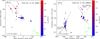 |
Fig. 1. View of the CH3OH maser features detected around G23.44−0.18 MM1 (left panel) and MM2 (right panel). The reference position is the estimated absolute position from Table 1. Triangles identify CH3OH maser features whose side length is scaled logarithmically according to their peak flux density (Table A.1). Maser local standard of rest radial velocities are indicated by color (the assumed velocity of the region is |

Only linearly polarized emission has been detected, in particular from six maser features associated with MM1 ( ) and from five associated with MM2 (
 ). The FRTM code (see Sect. 3) was able to fit all of them and the outputs of the code are reported in Cols. 9, 10, and 14 of Table A.1. We note that due to their high Pl the features G23.E25 and G23.E51 might be partially saturated. The estimated θ angles indicate that the magnetic field is perpendicular to the linear polarization vectors.
Considering the rms and the σs.−n. (see Table 1) for the strongest maser feature (G23.E03) we would have been able to detect circularly polarized emission only if PV > 1%, which is twice the typical fraction (PV ≈ 0.5%; e.g., Paper III).
4.2. G25.83−0.18
In Table A.2 we report the 46 CH3OH maser features detected towards G25.83−0.18 and named G258.E01–G258.E46. The very first VLBI distribution of these maser features is shown in Fig. 2, where we also report the red- and blue-shifted orientation, but not at the actual position, of the 13CO outflow (de Villiers et al. 2014). The maser features, in particular the northwestern group, are aligned NW–SE (PACH3OH = +51° ± 7°) without a clear velocity gradient. Their velocities, except for G258.E01 and G258.E28, are consistent with the red-shifted lobe of the outflow.
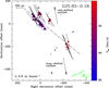 |
Fig. 2. View of the CH3OH maser features detected around G25.83−0.18 (Table A.2). Symbols are the same as in Fig. 1. The polarization fraction is in the range Pl = 2.3−9.7% (Table A.2). The assumed velocity of the YSO is |
Among the seven massive SFRs studied in the present work, G25.83−0.18 has the highest number of linearly polarized features (16 out of 46). The fractional linear polarization ranges from 2.3% to 9.7%, which is one of the highest measured so far. Although the high Pl indicates that five maser features might be partially saturated, we were able to fit all of the polarized maser features with the FRTM code. From the estimated θ angles (Col. 14 of Table A.2) the magnetic field is oriented perpendicular to the linear polarization vectors. No circular polarization was measured (PV < 0.9%).
4.3. G25.71−0.04
We identified 26 CH3OH maser features (named G257.E01–G257.E26 in Table A.3). Their complex distribution is shown in Fig. 3. Here, the orientation of the red- and blue-shifted lobes of the 13CO outflow are also displayed (de Villiers et al. 2014). The velocity range of 24 out of 26 CH3OH maser features (89 km s−1 < Vlsr < 100 km s−1) is within the velocity range of the blue-shifted lobe ( ; de Villiers et al. 2014), confirming their association with it.
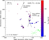 |
Fig. 3. View of the CH3OH maser features detected around G25.71−0.04 (Table A.3). Symbols are the same as in Fig. 1. The polarization fraction is in the range Pl = 0.4−1.6% (Table A.3). The assumed velocity of the YSO is |


We detected linearly polarized emission towards five CH3OH maser features (0.4% < Pl < 1.6%), among which G257.E12 also showed circular polarization (PV = 0.8%). The error-weighted intrinsic thermal linewidth,  , is one of the largest ever provided by the FRTM code, while the TbΔΩ values are within the typical estimated values for the 6.7 GHz CH3OH maser emission. Following Paper III we found for the features G257.E13 (offset =−71.456 mas; 125.005 mas) and G257.E19 (0 mas; 0 mas) that the magnetic field is parallel to the linear polarization vectors since |θ+−55°| < |θ− − 55°|, where θ± = θ ± ε±, and with ε± the errors associated with θ. For all the other maser features the magnetic field is perpendicular. The circularly polarized emission of G257.E12 was fitted with the FRTM code by including the corresponding ΔVi and TbΔΩ fit values obtained from the total and linearly polarized intensities. The fitted result is reported in Table A.3 and shown in Fig. 4. The nondetection of circular polarization for the very bright maser features G257.E13 and G257.E19 is likely due to the high σs.−n. (55 and 97 mJy beam−1, respectively). Considering the criterion 3σs.−n., we have upper limits of PV < 0.8% and <0.6% for G257.E13 and G257.E19, respectively.
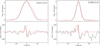 |
Fig. 4. Total intensity (I, upper panel) and circularly polarized intensity (V, lower panel) spectra for the CH3OH maser features named G257.E12 and G288.E19 (see Tables A.3, A.5). The thick red lines are the best-fit models of I and V emissions obtained using the adapted FRTM code (see Sect. 3). The maser features were centered on zero velocity. |
4.4. G28.31−0.39
Towards G28.31−0.39, we detected 13 CH3OH maser features (named G283.E01–G283.E13 in Table A.4). The Vlsr of eleven features ranges from 79.91 km s−1 to 83.23 km s−1, in accordance with  (de Villiers et al. 2014). The maser features G283.E12 and G283.E13 have higher velocities, Vlsr = 92.72 km s−1 and Vlsr = 93.81 km s−1, respectively, which are close to the highest velocity of the red-shifted lobe of the outflow (∼89 km s−1). In Fig. 5 the complex 3200 au × 2400 au distribution of the maser features, which resembles an X, is shown.
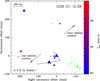 |
Fig. 5. View of the CH3OH maser features detected around G28.31−0.39 (Table A.4). Symbols are the same as in Fig. 1. The polarization fraction is in the range Pl = 1.6−4.3% (Table A.4). The assumed velocity of the YSO is |
The fit with the FRTM code of the two linearly polarized maser features, G283.E03 and G283.E10, provided for both of them that θ > 55°, i.e., that the magnetic field is perpendicular to the linear polarization vectors. Circular polarization has not been detected (PV < 0.5%).
4.5. G28.83−0.25
At VLBI scales we detected 21 6.7 GHz CH3OH maser features (named G288.E01–G288.E21 in Table A.5) linearly distributed (PACH3OH = −41° ± 10°; see Fig. 6) from southwest (the most red-shifted) to northeast (around systemic velocity  ; de Villiers et al. 2014). The maser features at the center of the linear distribution show the most blue-shifted velocities, in accordance with Cyganowski et al. (2009) and Fujisawa et al. (2014). The velocity distribution of the maser features reflects an almost perfect overlap of the red- and blue-shifted lobe emissions of the 13CO outflow (de Villiers et al. 2014). Therefore, it is difficult to associate the maser features with either the outflow or an accretion disk.
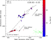 |
Fig. 6. View of the CH3OH maser features detected around G28.83−0.25 (Table A.5). Symbols are the same as in Fig. 1. The polarization fraction is in the range Pl = 0.5−3.3% (Table A.5). The assumed velocity of the YSO is |


We measured fractional linear polarization between 0.5% and 3.3% from six CH3OH maser features. For the brightest maser feature G288.E16, by fitting its polarized emission with the FRTM code, we found that  . This implies that the magnetic field is more likely parallel to the linear polarization vector of G288.E16 (see Paper III). For the other maser features this is instead perpendicular. Furthermore, we detected circularly polarized emission (PV = 0.6%) from G288.E19 that does not show linearly polarized emission. Hence, to model the circularly polarized emission we assumed that its emerging brightness temperature is equal to the error-weighted value ⟨TbΔΩ⟩ = 9.4 × 10⁸ K sr of the region; for the intrinsic thermal linewidth we determined that ΔVi = 1.1 km s−1 is the value that best fits the total intensity emission (see right panel of Fig. 4). The σs.−n. for the bright maser features G288.E16 and G288.E18 are 81 and 64 mJy beam−1, which imply PV < 0.8% and < 1.0%, respectively.
4.6. G29.96−0.02
We detected 34 6.7 GHz CH3OH maser features (named G29.E01–G29.E34 in Table A.6) towards the rotating disk of G29.96−0.02, distributed perpendicularly to the SiO jet from northeast to southwest (PACH3OH = +80° ± 3°, Fig. 7). Two of them (G29.E33 and G29.E34), the most northeastern, were previously undetected at VLBI scales (Sugiyama et al. 2008). The velocities of the maser features ranges from 95.65 km s−1 to 105.75 km s−1 without an ordered distribution along the major axis of the rotating disk. Even though the association of most of the maser features with the rotating disk is plausible, some of them might be associated with the outflowing gas. This hypothesis can be verified only by measuring their proper motions.
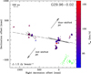 |
Fig. 7. View of the CH3OH maser features detected around G29.96−0.02 (Table A.6). Symbols are the same as in Fig. 1. The polarization fraction is in the range Pl = 1.4−5.7% (Table A.6). The assumed velocity of the YSO is |

Linearly polarized emission (Pl = 1.4%−5.7%) was measured towards four maser features grouped two by two: G29.E09 (the brightest) and G29.E12 towards the west and G29.E26 and G29.E30 towards the east. The west group shows Pl > 4% and an error-weighted linear polarization angle of ⟨ χ⟩west = +76° ±1°, while the east group shows Pl ≲ 2% and ⟨ χ⟩east = +49° ±6°. The total error-weighted linear polarization angle is ⟨ χ⟩ = + 62° ±17°. The FRTM code properly fits all of them and provided consistent outputs, though the TbΔΩ is higher, as expected, for the west group, which might be entering the saturated state. The angle between the magnetic field and the maser propagation direction is greater than 55° for all four maser features indicating that the magnetic field is perpendicular to the linear polarization vectors. No circularly polarized emission was detected (PV < 0.3%).
4.7. G43.80−0.13
With the EVN we were able to detect twice the number of 6.7 GHz CH3OH maser features previously detected by Sugiyama et al. (2008). These maser features are listed as G43.E01–G43.E18 in Table A.7, and are shown in Fig. 8 where the perpendicularity of their linear distribution (PACH3OH = −48° ± 5°) to the HCO+ outflow is clearly seen. The velocity range of the maser features (39.5 km s−1 < Vlsr < 43.2 km s−1) is blue-shifted with respect to the systemic velocity of the region ( , López-Sepulcre et al. 2010) and it is consistent with the range reported in Sugiyama et al. (2008). In particular, the velocities of the maser features located to the southeast (G43.E15–G43.E18) are closer to the systemic velocity, and the most blue-shifted are located towards the northeast.
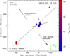 |
Fig. 8. View of the CH3OH maser features detected around G43.80−0.13 (Table A.7). Symbols are the same as in Fig. 1. The polarization fraction is in the range Pl = 1.1−4.4% (Table A.7). The assumed velocity of the YSO is |
Three maser features out of 18 showed linearly polarized emission with 1% < Pl < 4.5%, i.e., they are likely unsaturated. Despite this finding, the FRTM code was able to provide only an upper limit of ΔVi for G43.E04. The estimated θ angles indicate that the magnetic field is oriented perpendicular to the linear polarization vectors. No circularly polarized emission was detected, likely due to the weakness of the maser features (I < 6 Jy beam−1; PV < 0.8%).
5. Discussion
5.1. Magnetic field orientations
If the linearly polarized emission passes through a medium where a magnetic field is present before reaching the observer, its linear polarization vector suffers a rotation known as Faraday rotation. In the case of polarized CH3OH maser emission, two main Faraday rotations can affect the linear polarization vectors that we measure: internal rotation (Φi) and foreground Faraday rotation (Φf). An analysis of these two components of Faraday rotation was undertaken in the previous papers in the series (Papers I, II, and III); this analysis helps understand why we do not consider them important here. However, in Col. 2 of Table 4 we list Φf for each source.
The estimated orientation of the magnetic field6 in the seven massive SFRs under investigation here are separately discussed below.
G23.44–0.18. The magnetic fields around MM1 and MM2 are oriented SE–NW with error-weighted orientation of  and
and  . It should be noted that the CO outflow on the plane of the sky is oriented with an angle of
  and shows an opening angle of ∼30° (Ren et al. 2011). However, the velocity range of the masers both in MM1 and in MM2 falls between the velocity ranges of the LVC and HVC CO outflows indicating that the masers are not associated with either of them. The eastern maser group of MM2 shows a linear distribution perpendicular to the CO outflow (see Table 4) suggesting a possible disk structure, though the velocity distribution of the masers does not.
G25.83–0.18. The magnetic field is oriented with an angle on the plane of the sky of ⟨ΦB⟩ = − 67 ±7°, which is almost perpendicular both to the linear distribution of the 6.7 GHz CH3OH masers (PACH3OH = +51° ± 7°) and to the 13CO outflow ( , de Villiers et al. 2014).
G25.71–0.04. Taking into account the different orientation of the magnetic field with respect to the linear polarization vectors of the maser features, we measured an error-weighted magnetic field orientation of ⟨ΦB⟩ = − 80° ±43°, implying that it is aligned with the blue-shifted lobe of the 13CO outflow ( ; de Villiers et al. 2014). The location and velocities of the CH3OH masers also suggest that the masers probe the magnetic field along the blue-shifted lobe of the outflow.
G28.31–0.39. We were able to determine the orientation of the magnetic field on the plane of the sky from two blue-shifted CH3OH masers. Also in this case, the magnetic field (⟨ΦB⟩ = − 50° ±44°) is aligned with the 13CO outflow ( , de Villiers et al. 2014).
G28.83–0.25. Considering the different orientation of the magnetic field with respect to the linear polarization vector of G288.E16, the error-weighted orientation of the magnetic field on the plane of the sky is ⟨ΦB⟩ = + 58° ±59°. This is perpendicular to the linear distribution of the masers (PACH3OH = −41° ± 10°) and to the 13CO outflow (PACH3OH = −40°), even though the outflow is almost along the line of sight. Therefore, the interpretation of the morphology of the magnetic field is not straightforward.
G29.96–0.02. The magnetic field is oriented on the plane of the sky along the SiO jet ( , Cesaroni et al. (2017) with an angle of ⟨ΦB⟩ = − 29° ±17° and perpendicular to the rotating disk (Cesaroni et al. 2017). Considering separately the east and west group (⟨ΦB⟩east = −41° ±6° and ⟨ΦB⟩west = −14° ±1°), we note that the morphology of the magnetic field coincides with the morphology of the red-shifted lobe of the SiO jet near to the massive YSO (see Fig. 13 of Cesaroni et al. 2017).
G43.80–0.13. The orientation of the magnetic field (⟨ΦB⟩ = + 9° ±5°) derived from the masers, all of which belong to the most blue-shifted group, is misaligned by about 30° compared to the HCO+ outflow ( ; López-Sepulcre et al. 2010).
5.2. Magnetic field strength
Thanks to the work of Lankhaar et al. (2018), we are able to estimate a lower limit of B|| from the measurements of the Zeeman splitting of the 6.7 GHz CH3OH maser by assuming αZ = −0.051 km s−1 G−1 (Lankhaar et al. 2018). A direct measurement of B|| can indeed be only possible when the contribution of all eight hyperfine transitions to the 6.7 GHz CH3OH maser emission will be determined properly by modeling the pumping mechanism of the maser. However, by knowing the inclination of the magnetic field with respect to the line of sight (i.e., the θ angle), we can also estimate a lower limit for the magnetic field strength ( ; considering
  ). We were able to measure both B|| and B towards two of the seven massive YSOs reported in this work: G25.71−0.04 and G28.83−0.25.
G25.71–0.04. From the circularly polarized emission of G257.E12 we measured a Zeeman splitting of −3.1 ± 0.7 m s−1, which implies a magnetic field along the line of sight of B|| > 61 mG. By assuming θmin > 43° (see Col. 14 of Table A.3) the 3D magnetic field strength is B > 78 mG.
G28.83–0.25. The Zeeman splitting measured by modeling the circularly polarized emission of G288.E19 is ΔVZ = −1.1 ± 0.3 m s−1, for which we have B|| > 21 mG. Considering an error-weighted angle of  the 3D magnetic field is B > 28 mG. The 3D magnetic field measured from the CH3OH maser is four times larger than that measured from the OH maser (Bayandina et al. 2015). From the relation
  (Crutcher 1999), we determine that the CH3OH maser are arising from a gas with a density at least an order of magnitude higher than that of the OH maser. This agrees with the ranges of nH2 for the two maser species (e.g., Cragg et al. 2002).
From the estimated B values we can investigate the importance of the magnetic field in the high-mass star-forming process. If the ratio β between the thermal (ET) and the magnetic energies (EB) is lower than one (β < 1), the magnetic field dominates in the high-density CH3OH maser environment. Following Eq. (11) of Surcis et al. (2011a), we see that the ratio β also depends, in addition to the magnetic field, on the characteristics of the gas where the masers arise, namely on the number density of the gas (nH2) and on the kinetic temperature of the gas (Tk). Cragg et al. (2002, 2005) modeled the Class II CH3OH maser emissions and found that the masers arise when 105 cm−3 < nH2 < 109 cm−3 and 100 K < Tk < 200 K. Considering β = 1 we determined |Bcrit| values for all the possible combinations of the nH2 and Tk extremes (see Table 2). If |B| > |Bcrit| the magnetic field dominates over the thermal motions. In the case of G25.71−0.04 and G28.83−0.25 the magnetic field dominates the dynamics independently of the characteristics of the gas and on the specific dominating hyperfine transition.
|Bcrit| values for the ranges of nH2 and Tk.
In the past, we have reported erroneous values of Zeeman-splitting due to an error in the FRTM code (see Sect. 3). We report the corrected values of Zeeman-splitting with the corresponding lower limits of B|| and B in Table 3. The varying values of |B| measured from different maser features within the same source might indicate different gas properties in the massive SFR due either to the association of the CH3OH masers with different YSOs (e.g., W3(OH) and G24.78+0.08; Papers I and III) or to the different locations of the masers in the associated protostar (e.g., W51-e2 and G24.78+0.08-A1; Papers I and III). Nevertheless, if at least one of the masers detected towards a massive YSO provides |B| > 25 mG (see Table 2) we can assume that the magnetic field dominates there. The only sources for which we cannot determine whether the magnetic field dominates independently of the characteristics of the gas and on the specific dominating hyperfine transition are IRAS 06058+2138-IRS 1 and S255-IR (Paper II).
Magnetic fields measurements around massive YSOs determined by observing, with the EVN, the circularly polarized emission of 6.7 GHz CH3OH masers.
5.3. Updated statistical results
In Paper III, since we were at the midpoint of our project7, we updated our first statistical results reported in Paper II. Here, we would like to provide the updated statistical results based on seven more sources with respect to Paper III, i.e., 35 YSOs in total, also including the southern hemisphere sources reported in the literature (Paper II and references therein). Similarly to Papers II and III, we list in Table 4 the sources of the flux-limited sample analyzed so far for which we were able to measure the projection on the plane of the sky of the angles |PAoutflow−⟨ΦB⟩|, |PACH3OH − ⟨χ⟩|, and |PACH3OH − PAoutflow|, where PAoutflow is the orientation of the large-scale molecular outflow, ⟨ΦB⟩ is the error-weighted orientation of the magnetic field, PACH3OH is the orientation of the CH3OH maser distribution, and ⟨ χ⟩ is the error-weighted value of the linear polarization angles (for more details regarding Table 4, see the table notes and Paper III). In Table 5 we report the results of the Kolmogorov–Smirnov (K–S) test, which is a nonparametric test; here it is used to compare samples of angles (|PACH3OH − ⟨χ⟩|, |PACH3OH − PAoutflow|, and |PAoutflow − ⟨ΦB⟩|) with the random probability distribution (see Paper II for more details). Performing the statistical analysis we note that the probability that the angles |PACH3OH − ⟨χ⟩| are drawn from a random distribution is 28%8.
Comparison between position angle of magnetic field, CH3OH maser distribution, outflows, and linear polarization angles.
Results of Kolmogorov–Smirnov test.
For |PACH3OH −PAoutflow| and |PAoutflow − ⟨ΦB⟩| we measured probabilities similar to those reported in Paper III, these are 38% and 3% instead of 34% and 10% (Paper III), respectively. The updated results reinforce our previous finding: the magnetic field close to the YSO is preferentially oriented along the outflow axis.
6. Summary
We observed seven massive SFRs at 6.7 GHz in full polarization spectral mode with the EVN; our aim was to detect the linearly and circularly polarized emission of CH3OH masers. We detected linearly polarized emission towards all the regions and circularly polarized emission towards G25.71−0.04 and G28.83−0.25. We used the adapted FRTM code to model both the linear and the circular polarization of the masers. In particular, to estimate a lower limit of the magnetic field along the line of sight we assumed that the dominant hyperfine component, the one with the largest Einstein coefficient for stimulated emission, is F = 3 → 4 (Lankhaar et al. 2018). By analyzing the linearly polarized emission of the masers we were able to estimate the orientation of the magnetic field around eight massive YSOs (two are located within G23.44−0.18: MM1 and MM2). We found that the magnetic fields are aligned with the outflows (|PAoutflow − ⟨ΦB⟩| < 30°) in five YSOs (G23.44−0.18-MM2, G25.71−0.04, G28.31−0.39, G29.96−0.02, G43.80−0.13) and are perpendicular to the outflows in two YSOs (G25.83−0.18 and G28.83−0.25). The estimated magnetic field strengths along the line of sight for G25.71−0.04 and G28.83−0.25 are B|| > 61 mG and B|| > 21 mG, respectively. The magnetic field seems to dominate the dynamics of the gas in both YSOs.
We further increased the number of sources to 26, which is 80% of the flux-limited sample; the projected angles of the magnetic field and of the outflows of these sources are known. Comparing these angles, we confirm the statistical evidence that the magnetic fields around massive YSOs are preferentially oriented along the molecular outflows. In particular, the probability that the distribution of angles |PAoutflow − ⟨ΦB⟩| is drawn from a random distribution is lower (3%) than was reported in Paper III (10%).
μ = (M/Φ)/(M/Φ)crit, where (M/Φ) is the mass-to-magnetic flux ratio and  is the critical value of this ratio, where G is the gravitational constant (Tomisaka et al. 1988). The critical value indicates the maximum mass supported by the magnetic field (Tomisaka et al. 1988). The stronger the magnetic field, the lower μ.
The self-noise is high when the power contributed by the astronomical maser is a significant portion of the total received power (Sault 2012).
⟨ΦB⟩ is the mean error-weighted orientation of the magnetic field measured considering all the magnetic field vectors measured in a source. The weights are 1/ei, where ei is the error of the ith measured vector. The error on ⟨ΦB⟩ is the standard deviation. The position angle of the magnetic field vectors are measured with respect to the north, clockwise (negative) and counterclockwise (positive), as the PA of the outflows.
Acknowledgments
We wish to thank the referee S. Ellingsen for the useful suggestions that have improved the paper. W.H.T.V. acknowledges support from the European Research Council through consolidator grant 614264. A.B. acknowledges support from the National Science Centre, Poland, through grant 2016/21/B/ST9/01455. G.S., W.H.T.V., and H.J.van L. thank Hans Engelkamp and his team for their help in attempting the laboratory measurements of the Landé g-factor of the CH3OH molecule by using the 30 Tesla Magnet at the High Field Magnet Laboratory of the Radboud University in Nijmegen (The Netherlands). The European VLBI Network is a joint facility of independent European, African, Asian, and North American radio astronomy institutes. Scientific results from data presented in this publication are derived from the following EVN project code(s): ES072. The research leading to these results has received funding from the European Commission Seventh Framework Programme (FP/2007-2013) under grant agreement No. 283393 (RadioNet3).
References
- Andreev, N., Araya, E. D., Hoffman, I. M., et al. 2017, ApJS, 232, 29 [NASA ADS] [CrossRef] [Google Scholar]
- Araya, E. D., Hofner, P., Goss, W. M., et al. 2008, ApJS, 178, 330 [NASA ADS] [CrossRef] [Google Scholar]
- Banerjee, R., & Pudritz, R. E. 2007, ApJ, 660, 479 [NASA ADS] [CrossRef] [Google Scholar]
- Błaszkiewicz, L., & Kus, A. J. 2004, A&A, 413, 233 [NASA ADS] [CrossRef] [EDP Sciences] [Google Scholar]
- Bayandina, O. S., Val’tts, I. E., & Kurtz, S. E. 2015, Astron. Rep., 59, 998B [NASA ADS] [CrossRef] [Google Scholar]
- Beltrán, M. T., Olmi, L., Cesaroni, R., et al. 2013, A&A, 552, A123 [NASA ADS] [CrossRef] [EDP Sciences] [Google Scholar]
- Beuther, H., Zhang, Q., Bergin, E. A., et al. 2007, A&A, 468, 1045 [NASA ADS] [CrossRef] [EDP Sciences] [Google Scholar]
- Bonnell, I. A., Bate, M. R., Clarke, C. J., et al. 2001, MNRAS, 323, 785 [NASA ADS] [CrossRef] [Google Scholar]
- Braz, M. A., & Epchtein, N. 1983, A&AS, 54, 167 [NASA ADS] [Google Scholar]
- Breen, S. L., & Ellingsen, S. P. 2011, MNRAS, 416, 178 [NASA ADS] [Google Scholar]
- Breen, S. L., Fuller, G. A., Caswell, J. L., et al. 2015, MNRAS, 450, 4109 [NASA ADS] [CrossRef] [Google Scholar]
- Breen, S. L., Ellingsen, S. P., & Caswell, J. L. 2016, MNRAS, 459, 4066 [NASA ADS] [CrossRef] [Google Scholar]
- Bronfman, L., Nyman, L.-A., & May, J. 1996, A&AS, 115, 81 [NASA ADS] [Google Scholar]
- Brunthaler, A., Reid, M. J., Mente, K. M., et al. 2009, ApJ, 693, 424 [NASA ADS] [CrossRef] [Google Scholar]
- Caswell, J. L., Green, J. A., & Phillips, C. J. 2013, MNRAS, 431, 1180 [NASA ADS] [CrossRef] [Google Scholar]
- Cesaroni, R., Churchwell, E., Hofner, P., et al. 1994, A&A, 288, 903 [NASA ADS] [Google Scholar]
- Cesaroni, R., Hofner, P., Walmsley, C. M., et al. 1998, A&A, 331, 709 [NASA ADS] [Google Scholar]
- Cesaroni, R., Sánchez-Monge, Á., Beltrán, M. T., et al. 2017, A&A, 602, A59 [NASA ADS] [CrossRef] [EDP Sciences] [Google Scholar]
- Churchwell, E., Povich, M. S., Allen, D., et al. 2006, ApJ, 649, 759 [NASA ADS] [CrossRef] [Google Scholar]
- Cragg, D. M., Sobolev, A. M., & Godfrey, P. D. 2002, MNRAS, 331, 521 [NASA ADS] [CrossRef] [Google Scholar]
- Cragg, D. M., Sobolev, A. M., & Godfrey, P. D. 2005, MNRAS, 360, 533 [NASA ADS] [CrossRef] [Google Scholar]
- Crutcher, R. M. 1999, ApJ, 520, 706 [NASA ADS] [CrossRef] [Google Scholar]
- Cyganowski, C. J., Whitney, B. A., Holden, E., et al. 2008, AJ, 136, 2391 [NASA ADS] [CrossRef] [Google Scholar]
- Cyganowski, C. J., Brogan, C. L., Hunter, T. R., et al. 2009, ApJ, 702, 1615 [NASA ADS] [CrossRef] [Google Scholar]
- Cyganowski, C. J., Brogan, C. L., Hunter, T. R., et al. 2011, ApJ, 743, 56 [NASA ADS] [CrossRef] [Google Scholar]
- Dall’Olio, D., Vlemmings, W. H. T., Surcis, G., et al. 2017, A&A, 607, A111 [NASA ADS] [CrossRef] [EDP Sciences] [Google Scholar]
- De Buizer, J. M., Watson, A. M., Radomski, J. T., et al. 2002, ApJ, 564, L101 [NASA ADS] [CrossRef] [Google Scholar]
- de Villiers, H. M., Chrysostomou, A., Thompson, M. A., et al. 2014, MNRAS, 444, 566 [NASA ADS] [CrossRef] [Google Scholar]
- Fish, V. L., Reid, M. J., Argon, A. L., et al. 2005, ApJS, 160, 220 [NASA ADS] [CrossRef] [Google Scholar]
- Fujisawa, K., Sugiyama, K., Motogi, K., et al. 2014, PASJ, 66, 31 [NASA ADS] [Google Scholar]
- Girart, J. M., Torrelles, J. M., Estalella, R., et al. 2016, MNRAS, 462, 352 [NASA ADS] [CrossRef] [Google Scholar]
- Goddi, C., Surcis, G., Moscadelli, L., et al. 2017, A&A, 597, A43 [NASA ADS] [CrossRef] [EDP Sciences] [Google Scholar]
- Goldreich, P., Keeley, D. A., & Kwan, J. Y. 1973, ApJ, 179, 111 [NASA ADS] [CrossRef] [Google Scholar]
- Green, J. A., & McClure-Griffiths, N. M. 2011, MNRAS, 417, 2500 [NASA ADS] [CrossRef] [Google Scholar]
- Hennebelle, P., Commerçon, B., Joos, M., et al. 2011, A&A, 528, A72 [NASA ADS] [CrossRef] [EDP Sciences] [Google Scholar]
- Hoffman, I. M., Goss, W. M., Palmer, P., et al. 2003, ApJ, 598, 1061 [NASA ADS] [CrossRef] [Google Scholar]
- Hofner, P., & Churchwell, E. 1996, A&AS, 120, 283 [NASA ADS] [CrossRef] [EDP Sciences] [Google Scholar]
- Imai, H., Horiuchi, S., Deguchi, S., et al. 2003, ApJ, 595, 285 [NASA ADS] [CrossRef] [Google Scholar]
- Keimpema, A., Kettenis, M. M., Pogrebenko, S. V., et al. 2015, Exp. Astron., 39, 259 [NASA ADS] [CrossRef] [Google Scholar]
- Klassen, M., Pudritz, R. E., & Peters, T. 2012, MNRAS, 421, 2861 [NASA ADS] [CrossRef] [Google Scholar]
- Klassen, M., Kuiper, R., Pudritz, R. E., et al. 2014, ApJ, 797, 4 [NASA ADS] [CrossRef] [Google Scholar]
- Klassen, M., Pudritz, R. E., Kuiper, R., et al. 2016, ApJ, 823, 28 [NASA ADS] [CrossRef] [Google Scholar]
- Klessen, R. S., Peters, T., Banerjee, R., et al. 2011, IAU Symp., 270, 107 [NASA ADS] [Google Scholar]
- Krumholz, M. R., Klein, R. I., McKee, C. F., et al. 2009, Science, 323, 754 [NASA ADS] [CrossRef] [PubMed] [Google Scholar]
- Kuiper, R., Klahr, H., Beuther, H., et al. 2011, ApJ, 732, 20 [NASA ADS] [CrossRef] [Google Scholar]
- Kuiper, R., Yorke, H. W., & Turner, N. J. 2015, ApJ, 800, 86 [NASA ADS] [CrossRef] [Google Scholar]
- Kuiper, R., Turner, N. J., & Yorke, H. W. 2016, ApJ, 832, 40 [NASA ADS] [CrossRef] [Google Scholar]
- Kurtz, S., Churchwell, E., & Wood, D. O. S. 1994, ApJS, 91, 659 [NASA ADS] [CrossRef] [Google Scholar]
- Lankhaar, B., Vlemmings, W., Surcis, G., et al. 2018, Nat. Astron., 2, 145 [NASA ADS] [CrossRef] [Google Scholar]
- López-Sepulcre, A., Cesaroni, R., & Walmsley, C. M. 2010, A&A, 517, A66 [NASA ADS] [CrossRef] [EDP Sciences] [Google Scholar]
- Matsushita, Y., Machida, M. N., Sakurai, Y., et al. 2017, MNRAS, 470, 1026 [NASA ADS] [CrossRef] [Google Scholar]
- Matsushita, Y., Sakurai, Y., Hosokawa, T., et al. 2018, MNRAS, 475, 391 [NASA ADS] [CrossRef] [Google Scholar]
- McKee, C. F., & Tan, J. C. 2003, ApJ, 585, 850 [NASA ADS] [CrossRef] [MathSciNet] [Google Scholar]
- Minier, V., Booth, R. S., & Conway, J. E. 2000, A&A, 362, 1093 [NASA ADS] [Google Scholar]
- Minier, V., Booth, R. S., & Conway, J. E. 2002, A&A, 383, 614 [NASA ADS] [CrossRef] [EDP Sciences] [Google Scholar]
- Myers, A. T., McKee, C. F., Cunningham, A. J., et al. 2013, ApJ, 766, 97 [NASA ADS] [CrossRef] [Google Scholar]
- Myers, A. T., Klein, R. I., Krumholz, M. R., et al. 2014, MNRAS, 439, 3420 [NASA ADS] [CrossRef] [Google Scholar]
- Olmi, L., Cesaroni, R., Hofner, P., et al. 2003, A&A, 407, 225 [NASA ADS] [CrossRef] [EDP Sciences] [Google Scholar]
- Pestalozzi, M. R., Minier, V., & Booth, R. S. 2005, A&A, 432, 737 [NASA ADS] [CrossRef] [EDP Sciences] [Google Scholar]
- Peters, T., Klessen, A. S., Mac Low, M.-M., et al. 2010, ApJ, 725, 134 [NASA ADS] [CrossRef] [Google Scholar]
- Peters, T., Banerjee, R., Klessen, R. S., et al. 2011, ApJ, 729, 72 [NASA ADS] [CrossRef] [Google Scholar]
- Peters, T., Klaassen, P. D., Mac Low, M.-M., et al. 2012, ApJ, 760, 91 [NASA ADS] [CrossRef] [Google Scholar]
- Peters, T., Klaassen, P. D., Mac Low, M.-M., et al. 2014, ApJ, 788, 14 [NASA ADS] [CrossRef] [Google Scholar]
- Pillai, T., Kauffmann, J., Wyrowski, F., et al. 2011, A&A, 530, A118 [NASA ADS] [CrossRef] [EDP Sciences] [Google Scholar]
- Ren, J. Z., Liu, T., Wu, Y., et al. 2011, MNRAS, 415, L49 [NASA ADS] [CrossRef] [Google Scholar]
- Sanna, A., Reid, M. J., Menten, K. M., et al. 2014, ApJ, 781, 108 [NASA ADS] [CrossRef] [Google Scholar]
- Sanna, A., Moscadelli, L., Surcis, G., et al. 2017, A&A, 603, 94 [Google Scholar]
- Sarma, A. P., Troland, T. H., Romney, J. D., et al. 2008, ApJ, 674, 295 [NASA ADS] [CrossRef] [Google Scholar]
- Sault, R. J. 2012, EVLA Memo 159 [Google Scholar]
- Seifried, D., Banerjee, R., Klessen, R. S., et al. 2011, MNRAS, 417, 1054 [NASA ADS] [CrossRef] [Google Scholar]
- Seifried, D., Pudritz, R. E., Banerjee, R., et al. 2012, MNRAS, 422, 347 [NASA ADS] [CrossRef] [Google Scholar]
- Seifried, D., Banerjee, R., Pudritz, R. E., et al. 2015, MNRAS, 446, 2776 [NASA ADS] [CrossRef] [Google Scholar]
- Sugiyama, K., Fujisawa, K., Doi, A., et al. 2008, PASJ, 60, 23 [NASA ADS] [Google Scholar]
- Surcis, G., Vlemmings, W. H. T., Dodson, R., et al. 2009, A&A, 506, 757 [NASA ADS] [CrossRef] [EDP Sciences] [Google Scholar]
- Surcis, G., Vlemmings, W. H. T., Torres, R. M., et al. 2011a, A&A, 533, A47 [NASA ADS] [CrossRef] [EDP Sciences] [Google Scholar]
- Surcis, G., Vlemmings, W. H. T., Curiel, S., et al. 2011b, A&A, 527, A48 [NASA ADS] [CrossRef] [EDP Sciences] [Google Scholar]
- Surcis, G., Vlemmings, W. H. T., & van Langevelde, H. J. 2012, A&A, 541, A47 (Paper I) [NASA ADS] [CrossRef] [EDP Sciences] [Google Scholar]
- Surcis, G., Vlemmings, W. H. T., & van Langevelde, H. J. 2013, A&A, 556, A73 (Paper II) [NASA ADS] [CrossRef] [EDP Sciences] [Google Scholar]
- Surcis, G., Vlemmings, W. H. T., van Langevelde, H. J., et al. 2014a, A&A, 565, L8 [NASA ADS] [CrossRef] [EDP Sciences] [Google Scholar]
- Surcis, G., Vlemmings, W. H. T., van Langevelde, H. J., et al. 2014b, A&A, 563, A30 [NASA ADS] [CrossRef] [EDP Sciences] [Google Scholar]
- Surcis, G., Vlemmings, W. H. T., & van Langevelde, H. J. 2015, A&A, 578, A102 (Paper III) [NASA ADS] [CrossRef] [EDP Sciences] [Google Scholar]
- Szymczak, M., & Gérard, E. 2004, A&A, 414, 235 [NASA ADS] [CrossRef] [EDP Sciences] [Google Scholar]
- Szymczak, M., Olech, M., Sarniak, R., et al. 2018, MNRAS, 474, 219 [NASA ADS] [CrossRef] [Google Scholar]
- Tan, J. C., Beltrán, M. T., & Caselli, P. 2014, Protostars and Planets VI, 149 [Google Scholar]
- Thompson, M. A., Hatchell, J., Walsh, A. J., et al. 2006, A&A, 453, 1003 [NASA ADS] [CrossRef] [EDP Sciences] [Google Scholar]
- Tomisaka, K., Ikeuchi, S., & Nakamura, T. 1988, ApJ, 335, 239 [NASA ADS] [CrossRef] [Google Scholar]
- Towner, A. P. M., Brogan, C. L., Hunter, T. R., et al. 2017, ApJ, 136, 2391 [Google Scholar]
- Vaidya, B., Fendt, C., Beuther, H., et al. 2011, ApJ, 742, 56 [NASA ADS] [CrossRef] [Google Scholar]
- Vlemmings, W. H. T. 2008, A&A, 484, 773 [NASA ADS] [CrossRef] [EDP Sciences] [Google Scholar]
- Vlemmings, W. H. T., Diamond, P. J., van Langevelde, H. J., et al. 2006, A&A, 448, 597 [NASA ADS] [CrossRef] [EDP Sciences] [Google Scholar]
- Vlemmings, W. H. T., Surcis, G., Torstensson, K. J. E., et al. 2010, MNRAS, 404, 134 [NASA ADS] [Google Scholar]
- Vlemmings, W. H. T., Torres, R. M., & Dodson, R. 2011, A&A, 529, A95 [NASA ADS] [CrossRef] [EDP Sciences] [Google Scholar]
- Walsh, A. J., Hyland, A. R., Robinson, G., et al. 1997, MNRAS, 291, 261 [NASA ADS] [CrossRef] [Google Scholar]
- Walsh, A. J., Burton, M. G., Hyland, A. R., et al. 1998, MNRAS, 301, 640 [NASA ADS] [CrossRef] [Google Scholar]
- Walsh, A. J., Macdonald, G. H., Alvey, N. D. S., et al. 2003, A&A, 410, 597 [NASA ADS] [CrossRef] [EDP Sciences] [Google Scholar]
- Wardle, J. F. C., & Kronberg, P. P. 1974, ApJ, 194, 249 [NASA ADS] [CrossRef] [Google Scholar]
- Wood, D. O. S., & Churchwell, E. 1989, ApJS, 69, 831 [NASA ADS] [CrossRef] [Google Scholar]
- Wu, Y. W., Sato, M., Reid, M. J., et al. 2014, A&A, 566, A17 [NASA ADS] [CrossRef] [EDP Sciences] [Google Scholar]
- Yorke, H. W., & Richling, S. 2002, Rev. Mex. Astron. Astrophys., 12, 92 [NASA ADS] [Google Scholar]
- Zhang, Q., Qiu, K., Girart, J. M., et al. 2014a, ApJ, 792, 116 [NASA ADS] [CrossRef] [Google Scholar]
- Zhang, B., Moscadelli, L., Sato, M., et al. 2014b, ApJ, 781, 89 [NASA ADS] [CrossRef] [Google Scholar]
Appendix A: Additional tables
In Tables A.1–A.7 we list the parameters of all the CH3OH maser features detected toward the seven massive SFRs observed with the EVN and reported in this work. The tables are organized as follows. In Col. 1 we give the name of the feature, and only in Table A.1 the associated region is reported in Col. 1B. The positions, Cols. 2 and 3, refer to the maser feature used for self-calibration. From Cols. 4 to 6 we give the peak flux density, the LSR velocity (Vlsr), and the FWHM (ΔνL) of the total intensity spectra of the maser features that are obtained using a Gaussian fit. The mean linear polarization fraction (Pl) and the mean linear polarization angles (χ) are measured across the spectrum, and are listed in Cols. 7 and 8. The outcomes of the adapted FRTM code are listed in Cols. 9 (intrinsic thermal linewidth), 10 (emerging brightness temperature), and 14 (angle between the magnetic field and the maser propagation direction). The errors were determined by analyzing the full probability distribution function. The value of θ in bold indicates that |θ+ − 55°| < |θ− − 55°|, i.e., the magnetic field is assumed to be parallel to the linear polarization vector (see Papers I–III). Finally, the circular polarization fraction (PV), the Zeeman splitting (ΔVZ), and the lower limit of the magnetic field strength along the line of sight (B||) determined by fitting the V Stokes spectra by using the best-fitting results (ΔVi and TbΔΩ) and the Landé g-factors calculated by Lankhaar et al. (2018) for the hyperfine transition F = 3 → 4 are listed in Cols. 11, 12, and 13. The tables are only available at the CDS.
All Tables
Magnetic fields measurements around massive YSOs determined by observing, with the EVN, the circularly polarized emission of 6.7 GHz CH3OH masers.
Comparison between position angle of magnetic field, CH3OH maser distribution, outflows, and linear polarization angles.
All Figures
|
Fig. 1. View of the CH3OH maser features detected around G23.44−0.18 MM1 (left panel) and MM2 (right panel). The reference position is the estimated absolute position from Table 1. Triangles identify CH3OH maser features whose side length is scaled logarithmically according to their peak flux density (Table A.1). Maser local standard of rest radial velocities are indicated by color (the assumed velocity of the region is |
| In the text | |
|
Fig. 2. View of the CH3OH maser features detected around G25.83−0.18 (Table A.2). Symbols are the same as in Fig. 1. The polarization fraction is in the range Pl = 2.3−9.7% (Table A.2). The assumed velocity of the YSO is |
| In the text | |
|
Fig. 3. View of the CH3OH maser features detected around G25.71−0.04 (Table A.3). Symbols are the same as in Fig. 1. The polarization fraction is in the range Pl = 0.4−1.6% (Table A.3). The assumed velocity of the YSO is |
| In the text | |
|
Fig. 4. Total intensity (I, upper panel) and circularly polarized intensity (V, lower panel) spectra for the CH3OH maser features named G257.E12 and G288.E19 (see Tables A.3, A.5). The thick red lines are the best-fit models of I and V emissions obtained using the adapted FRTM code (see Sect. 3). The maser features were centered on zero velocity. |
| In the text | |
|
Fig. 5. View of the CH3OH maser features detected around G28.31−0.39 (Table A.4). Symbols are the same as in Fig. 1. The polarization fraction is in the range Pl = 1.6−4.3% (Table A.4). The assumed velocity of the YSO is |
| In the text | |
|
Fig. 6. View of the CH3OH maser features detected around G28.83−0.25 (Table A.5). Symbols are the same as in Fig. 1. The polarization fraction is in the range Pl = 0.5−3.3% (Table A.5). The assumed velocity of the YSO is |
| In the text | |
|
Fig. 7. View of the CH3OH maser features detected around G29.96−0.02 (Table A.6). Symbols are the same as in Fig. 1. The polarization fraction is in the range Pl = 1.4−5.7% (Table A.6). The assumed velocity of the YSO is |
| In the text | |
|
Fig. 8. View of the CH3OH maser features detected around G43.80−0.13 (Table A.7). Symbols are the same as in Fig. 1. The polarization fraction is in the range Pl = 1.1−4.4% (Table A.7). The assumed velocity of the YSO is |
| In the text | |
Current usage metrics show cumulative count of Article Views (full-text article views including HTML views, PDF and ePub downloads, according to the available data) and Abstracts Views on Vision4Press platform.
Data correspond to usage on the plateform after 2015. The current usage metrics is available 48-96 hours after online publication and is updated daily on week days.
Initial download of the metrics may take a while.