| Issue |
A&A
Volume 623, March 2019
|
|
|---|---|---|
| Article Number | A107 | |
| Number of page(s) | 9 | |
| Section | Stellar atmospheres | |
| DOI | https://doi.org/10.1051/0004-6361/201834516 | |
| Published online | 13 March 2019 | |
Spot evolution in the eclipsing binary CoRoT 105895502
Hamburger Sternwarte, Universität Hamburg,
Gojenbergsweg 112,
21029
Hamburg,
Germany
e-mail: stefan.czesla@hs.uni-hamburg.de
Received:
26
October
2018
Accepted:
28
January
2019
Stellar activity is ubiquitous in late-type stars. The special geometry of eclipsing binary systems is particularly advantageous to study the stellar surfaces and activity. We present a detailed study of the 145 d CoRoT light curve of the short-period (2.17 d) eclipsing binary CoRoT 105895502. By means of light-curve modeling with Nightfall, we determine the orbital period, effective temperature, Roche-lobe filling factors, mass ratio, and orbital inclination of CoRoT 105895502 and analyze the temporal behavior of starspots in the system. Our analysis shows one comparably short-lived (≈40 d) starspot, remaining quasi-stationary in the binary frame, and one starspot showing prograde motion at a rate of 2.3° day−1, whose lifetime exceeds the duration of the observation. In the CoRoT band, starspots account for as much as 0.6% of the quadrature flux of CoRoT 105895502, however we cannot attribute the spots to individual binary components with certainty. Our findings can be explained by differential rotation, asynchronous stellar rotation, or systematic spot evolution.
Key words: binaries: eclipsing / stars: activity / stars: individual: CoRoT 105895502
© ESO 2019
1 Introduction
Binary stars are numerous in the Galaxy (e.g., Raghavan et al. 2010; Yuan et al. 2015). Among the binaries, eclipsing systems are particularly valuable targets because they allow to study a plethora of stellar properties such as effective temperatures, masses, radii, and limb darkening parameters (e.g., Kjurkchieva et al. 2016). For a number of prominent eclipsing binaries such as AR Lac, observational records have been accumulated reaching back more than 100 yr (e.g., Siviero et al. 2006). Consequently, eclipsing binaries are ideal targets to put theories of stellar structure and evolution to the test (e.g., Ribas 2006; Parsons et al. 2018).
In close binary systems, stellar rotation and orbital motion are expected to become synchronized by tidal interaction (Zahn & Bouchet 1989). As discussed in a review by Mazeh (2008), observations of late-type stars in the pre-main sequence stage by Marilli et al. (2007) and in young open clusters by Meibom et al. (2006) show tidal synchronization for orbital periods of less than 10 days already at a few hundred millions years. Consequently, high rotation rates are maintained in such systems. According to the rotation–activity paradigm (cf., Pizzolato et al. 2003), this entails high activity levels, of which starspots are a prominent manifestation. Starspots can be used to study stellar rotation and its latitudinal dependence using spectroscopy (e.g., Kővári et al. 2017), photometry (e.g., Huber et al. 2010; Nagel et al. 2016; Santos et al. 2017), or both.
The space-based photometry provided by the CoRoT (Convection, Rotation, and planetary Transits, Auvergne et al. 2009) and Kepler satellites comprises a rich reservoir of eclipsing binary light curves (e.g., Matson et al. 2016). In contrast to ground-based data, neither the day–night cycle nor atmospheric turbulence interfere with the observations of these satellites, which allows for high-quality, uninterrupted photometric time series to be obtained, covering many months and years.
2 Target, observation, and data reduction
CoRoT 105895502 is an active eclipsing binary system (2MASS J18431107 + 0611448, Gaia DR2 4285571561155175424). Based on ground-based observations with the Berlin Exoplanet Search Telescope II (BEST II) located in Chile, Kabath et al. (2009) classified CoRoT 105895502 as an eclipsing binary system of Algol type. Further information on the system is given in Table 1. We here adopt the effective temperature estimate provided by Gaia. The value is probably affected by the binary nature of the target, which is not resolved. For main sequence stars, the quoted effective temperature corresponds to a late G spectral type with a mass of about 0.92 M⊙ (Pecaut & Mamajek 2013).
The CoRoT light curve of CoRoT 105895502 was obtained between Mar 31 and Sept 8, 2008, in the context of the second long run targeting the Galactic Center (LRc02) and spans approximately 145 d. The light curve shows strong eclipses of alternating depth with a shallower secondary eclipse being indicative of a cooler secondary star with lower surface brightness. The light curve shows variable out-of-eclipse modulation attributable to ellipsoidal variations and an evolving starspot pattern (see Fig. 1). CoRoT obtained a second light curve in July 2011, covering only 5 d. Both light curves were observed with a temporal sampling of 32 s. We downloaded the data from the public CoRoT N2 data archive. As the short 2011 light curve is only used in the determination of the ephemeris in our analysis, we focus on the long-run light curve in the following.
A bi-prism installed in front of the exoplanet CCD provides three color bands dubbed red, green, and blue. However, their spectral coverage remains uncalibrated, and therefore in this study we rely on the so-called white flux, that is, the sum of the three color channels. Further, we only accept measurements marked as valid by the standard pipeline (STATUS = 0), which causes the conspicuous lack of data around 3090 HCJD1 (see Fig. 1). Factors leading to the invalidation of flux measurements comprise the detection of cosmic particle impacts, detector hot pixels, and crossing of the South Atlantic Anomaly. Because the resulting light curve shows a number of suspicious, isolated upward outliers, we carry out an outlier rejection. In particular, we calculate the difference between consecutive data points and disregard those showing an upward jump exceeding 15 times the standard deviation of the noise compared to their predecessor. With this procedure, we reject a total of 131 data points, corresponding to only about 0.04% of the data set. Notably, we find no downward outliers in the light curve.
After these reduction steps, the light curve still exhibits some conspicuous, fast changes in the flux (jumps), which we consider instrumental rather than physical in nature. By visual inspection, we identified four such jumps, which occur at about 3031.385, 3087.573, 3102.532, and 3113.05 HCJD. To correct these jumps, we take advantage of the periodic nature of the light-curve modulation, showing only relatively weak variation between consecutive epochs (i.e., binary revolutions). Specifically, we remove the data points likely affected by the jump process and adjust the level of the following light-curve segment by multiplication with a factor, determined by considering the flux ratio between thepre- and post-jump phases observed during the preceding and following epochs. An example of the correction isshown in Fig. 2, and the entire revised white-light curve is shown in Fig. 1.
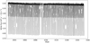 |
Fig. 1 Revised white light curve of CoRoT 105895502. |
Parameters of CoRoT 105895502.
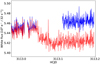 |
Fig. 2 Excerpt of the light curve around a jump before correction (red, dashed) and the jump-corrected light curve (blue, solid) after flux level adjustment and removal of likely affected data points. |
3 Properties of the light curve
The light curve displayed in Fig. 1 shows periodic variability with distinct transits. With a depth of about 28%, the primary eclipse is more than twice as deep as the secondary eclipse during which the observed flux drops by about 11%, which is indicative ofa cooler secondary component.
3.1 Orbital ephemeris
We determine the orbital period and a reference time for the eclipses by fitting the central one-hour section of both the primary and secondary eclipse light curves using a parabola and estimate the instant of minimum flux based on this model. Specifically, we use a by-eye estimate of the ephemeris as a starting solution, determine a preliminary instant of minimum flux by a fit to the data points no further than half an hour from the guessed position, and finally repeat the process using the preliminary position as a starting solution. With this procedure, we obtain the instants of minimum flux as a function of orbital revolution or, equivalently, epoch with respect to the reference time.
We next determine the orbital period using a linear fit to the instants of primary eclipse. The resulting period and reference time are given in Table 2 and the residuals are shown in Fig. 3; note that two additional primary eclipses as well as one secondary eclipse at epochs 533 and 534 constrain the ephemeris but are not shown here. The error was estimated using the jackknife procedure, which is a resampling technique (Efron & Stein 1981). To estimate jackknife errors, we repeat the analysis for all subsamples of data, which can be obtained by removing a single data point from the original set. The uncertainty of the best-fit value can then be estimated from the width of the thus-obtained distribution of parameter estimates.
While the secondary and primary eclipses are expected to show identical periods, the phase offset is not necessarily 0.5 if the binary orbit is not circular. In Fig. 3, we also show the residuals of the secondary eclipse times with respect to the primary ephemeris, which show a systematic offset compared to the nominal value of 0.5 valid for a circular orbit. Therefore, we set up a model with three free parameters, namely the reference time, the orbital period, and the phase offset of the secondary eclipse, and fit the parameters to the primary and secondary eclipse times. The resulting values are given in Table 2. While reference time and orbital period are consistent with those determined from the primary eclipse timing to within the uncertainty, a significant phase offset is found, corresponding to an average lag of 49 ± 4 s in the secondary eclipse time with respect to the prediction of a circular orbit; uncertainties are again derived using the jackknife.
The scatter in the residuals corresponding to the secondary eclipse times is larger and also appears to show systematic variation around epoch 20. While the larger scatter may be related to the smaller curvature of the secondary eclipse light curve compared to the center of the primary eclipse, the systematic variation is probably attributable to occulted starspots on the secondary component, making the timing of the primary eclipses more reliable. In the following analysis, we rely on the ephemeris derived from the combined model with a phase offset.
Based on the delay of the secondary eclipse, a value of 4 × 10⁻⁴ is obtained for the combination of eccentricity and argument of periastron, e cos (ω), which is also a lower limit for the eccentricity (e.g., Matson et al. 2016). Owing to the ellipsoidal variation and the effect of starspots, a difference inthe duration of the eclipses is hard to determine accurately. Assuming a conservative by-eye upper limit of 600 s, an eccentricity in excess of 1.8% can be ruled out however. We note that a fraction of the delay will be contributed by the light travel time effect (e.g., Kaplan 2010), causing a delay, ΔtLT, of
 (1)
(1)
Here, q is the binary mass ratio and K2 (in km s−1) is the radial-velocity semi-amplitude of the secondary component, both of which are unknown. Conservatively assuming 100 km s−1 for K2 and a mass ratio of 0.5, we estimate ΔtLT ≾ 10 s in our case.
Fit results for the ephemeris.
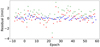 |
Fig. 3 Residuals of estimated eclipse times with respect to linear ephemeris for primary (blue dots) and secondary (red triangles) eclipses. Green crosses indicate the residuals of the secondary eclipse times with respect to the ephemeris derived from the primary eclipse timing. |
3.2 Evolution of the noise level
To prepare the modeling, we study the noise behavior of the light curve. In particular, we employ the βσ procedure by Czesla et al. (2018). If the signal were constant, an estimate of the sample standard deviation of the data would immediately yield the noise level. This is no longer true when there is considerable intrinsic variation in the signal, as in this case. The idea behind the βσ technique is to estimate the standard deviation of the noise, σ, by studyingthe distribution of numerical derivatives of the data (the β sample). In this way, the impact of intrinsic variation on the noise-level estimation can be minimized. For example, the difference between anypair of consecutive data points can be used to construct a sample of first-order derivatives, which will not be affected by a signal, varying only weakly between consecutive data points. In this case, we opted for second-order numerical derivatives and skippedevery second data point in the calculation of the derivatives to avoid potential correlation. Thus, we obtained the standard deviation of the noise for all epochs comprising more than 100 data points. Finally, we calculate the signal-to-noise ratio (S/N) by dividing the mean level of the light curve in each epoch by the noise level.
The evolution of the S/N is shown in Fig. 4. The S/N remains relatively constant between about 600 and 650 until around epoch 30. It then continuously decreases, indicating a loss of quality in the observations.
3.3 Light curve asymmetry
The light curve shows distinct time-variable modulation between the transits, which is characteristic of ellipsoidal variations and an evolving starspot configuration (e.g., Strassmeier 2009). While it seems improbable that there is any epoch without a contributionof starspots to the light curve, their impact differs among the various observed epochs. In view of the light-curve-modeling process, it is helpful to identify epochs for which some information on the instantaneous starspot configuration can be derived from more fundamental considerations. Here, we attempt to employ symmetry to identify such epochs.
We refer to two viewing geometries as equivalent if they can be transformed into each other by reflections or rotations in the plane of the sky. Such configurations therefore yield the same observed flux if Doppler boosting is neglected. Assuming a circular orbit, an aligned system, and the absence of starspots, the viewing geometry is equivalent for all instances Tt + τ and Tt − τ, where Tt is the center of any primary or secondary eclipse and τ is some time offset. It therefore follows for the observed flux, f(t), that
 (2)
(2)
The above relation continues to hold when starspots are added, if these are symmetric with respect to the plane generated by the vector connecting the stars and the orbit normal. By quantifying the accuracy of the relation, we can therefore identify epochs with a bona-fide symmetric starspot configuration.
In practice, we went through all observed epochs and divided the orbital phase intervals ϕa = 0.05–0.45 and ϕb = 0.55–0.95 into 20 equidistant bins each. The phase intervals are chosen such that the eclipses are excluded. We then defined the symmetry coefficient, cs, as
 (3)
(3)
where ai and bi denote the mean value of the data points in the ith bin in the phase intervals ϕa and ϕb and σi denotes the standard deviation of the sample mean of the data points in the respective bin. The thus-defined symmetry coefficient is shown as a function of epoch in Fig. 5.
The symmetry coefficient assumes a minimum for a symmetric light curve. According to Fig. 5 a particularly symmetric period was observed between epochs 40 and 50, which we attribute to a special starspot configuration. The lowest value of the symmetry coefficient is obtained for epoch 47 for which we find a numerical value of 135. Under the null hypothesis of identical expectations in all bins ai and bi (and normal errors), cs follows a χ2 -distribution with 20 degrees of freedom. The null can therefore be formally rejected at high significance, even for the most symmetric configuration observed according to the above condition.
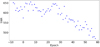 |
Fig. 4 The S/N as a function of epoch. |
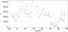 |
Fig. 5 The asymmetry coefficient as a function of epoch. |
4 Light-curve modeling
To model the light curve, we use the open source Nightfall code developed by one of the authors (R.W.). Here, we use version 1.88 (released Nov 2015). Nightfall models stars as equipotential surfaces of the Roche potential, using the geometric setup described by Djurašević (1992). The bolometric correction for mutual reflection follows the prescription by Hendry & Mochnacki (1992). The correction is calculated by an iterative procedure, and we use two iterations here after verifying that this suffices for the required accuracy. For the gravity-brightening exponent of convective stars, Nightfall uses the results from Claret (2000a), which provide a smooth transition to the von Zeipel (1924) exponent for radiative stars. For temperatures below 9800 K (as is the case here), model fluxes are based on PHOENIX models for solar abundances (Hauschildt & Baron 1999; Hauschildt et al. 2003). Limb darkening coefficients are taken from Claret (2000b). Nightfall provides tables of pre-computed band fluxes integrated over the supported filter bandpasses and interpolates in effective temperature Teff, but not in surface gravity logg, hence, we use a value of logg = 4.0 for both stars. To account for Doppler boosting, Nightfall applies a correction according to Eq. (3) in van Kerkwijk et al. (2010). The actual CoRoT passband is relatively broad (Auvergne et al. 2009). As CoRoT registers about 78% of the signal of CoRoT 105895502 in its so-called red color band (which remains uncalibrated, however), we use the R-band model fluxes to represent the light curve in our modeling with Nightfall.
Nightfall can take into account circular spots on both of the binary components. The spots are described by their stellar longitude and latitude, their radius, and a dimming factor, which specifies the ratio between starspot and photospheric effective temperature. To alleviate the effect of the notorious degeneracy between starspot radius and dimming factor in the modeling, we here consider only spots with a fixed radius of 20°. By opting for a large starspot radius, we simultaneously minimize effects related to the surface discretization on the objective function (i.e., χ2) in the minimization process.
The convention of stellar longitude adopted by Nightfall is shown in Fig. 6. The starspot latitude is often also rather ill-constrained in light-curve inversion problems because it is strongly degenerated with other properties, specifically the dimming factor and radius in our case. We therefore also fix the starspot latitude such that starspots are centered on the stellar equator. We note that the eclipses are particularly informative phases for breaking this degeneracy, however our modeling is focused on the inter-eclipse phases.
The assumption of large, circular spots is a simplification adopted only for modeling purposes. On the Sun, individual spots are typically much smaller, although they frequently appear in groups (e.g., Bogdan et al. 1988). Although the stars studied here are considerably more active than the Sun, their surfaces are also most likely covered by an ensemble of spots following some size distribution rather than giant monolithic spots. However, the small-scale structure remains unresolved in our light-curve modeling. As shown by Jeffers (2005) and Özavcı et al. (2018) the model spots absorb the combined effect of the longitudinally asymmetric part of the starspot configuration. Özavcı et al. (2018) specifically use the term “spot cluster” to underline this fact. While we stay with the spot nomenclature in the following, the approximative nature of the model should be kept in mind.
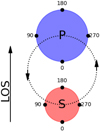 |
Fig. 6 Convention of stellar longitude used in Nightfall. |
4.1 Spot quadrature depression
The impact of a starspot at a given position on the model light curve is determined by the dimming factor and the spot radius. Because of the strong degeneracy, usually only some combination of these quantities is constrained in the modeling. Even after we break this degeneracy (not resolve it of course) by fixing the radius, the interpretation of the dimming factor in terms of its impact on the light-curve model remains somewhat intricate. Therefore, we here define a quantity, which can serve as a more direct measure of the spot impact on the model light curve.
When a single spot is put at a stellar longitude of 90° (and zero latitude), it faces the observer at quadrature between secondary and primary eclipse. Here, we define the spot quadrature depression (SQD) as the relative loss of flux caused by a spot of a given dimming factor and radius, located at a stellar longitude of 90°, during quadrature phase compared to an unspotted model. The SQD is a measure of the spot impact on the model, combining the effects of the dimming factor and the radius. It is also comparable for spots on the primary and secondary component, whose effective temperatures differ, further complicating the interpretation of the dimming factors.
4.2 The fundamental binary parameters
Our goal here is to determine the fundamental system parameters, namely the orbit inclination (iorb), the mass ratio (q), the Roche lobe filling factors for primary and secondary (fP and fS), and the effective temperatures (Teff,P and Teff,S), which we consider constant throughout the observed light curve. In addition, we allow for a free normalization factor in the model to represent the unknown absolute flux level, which we consider a nuisance parameter in the modeling. As the light-curve modeling is mainly sensitive to the ratio of surface brightnesses in the observed band, we fix the effective temperature, Teff,P, of the primary star to 5500 K in accordance with the Gaia results (Table 1) and further assume a value of four for log (g) for both components of the system.
Time-dependent starspot patterns represent a nuisance in the context of determining the binary parameters, because they add more free parameters to the problem. In Sect. 3.3, we concluded that it is unlikely that the light curve is free from starspot contributions during any observed epoch but found that epoch 47 displays the most symmetric light curve. While the true number of starspots remains unknown, we are confident that they were located close to the central plane during this epoch and that their combined effect can therefore be absorbed by a single circular spot in the modeling.
In Fig. 7 we show the observed CoRoT light curve during epoch 47 along with our best-fit model and the residuals. The best-fit parameters are listed in Table 3. Formally, we obtain a χ2 value of 5075.8 with 5158 degrees of freedom and, consequently, a reduced χ2 value of 0.98. Nonetheless, some systematic residuals can be identified, which are associated with the beginning of ingress and the end of egress. This may be attributable to the adopted description of limb-darkening or unaccounted-for contributions of potentially occulted starspots. To test for the randomness of the residuals, we carried out a Wald-Wolfowitz runs test on their signs (Wald & Wolfowitz 1940; Bradley 1968). In particular, we consider here any consecutive sequence of two or more residuals with the same sign a “run”. We find a total of 1283 such runs in the residuals of the fit. Under the null hypothesis of independent residuals with equal expectation of being positive or negative, we find an expected number of 1291 ± 18 runs by means of a simulation, which provides no evidence against the null. Therefore, we find both the χ2 and the runs test to be consistent with an acceptable fit result.
To verify that a model without a starspot does not yield an equally acceptable result, we repeat the minimization without a starspot, which increases the number of degrees of freedom by two. With this approach, however, we end up with a best-fit reduced χ2 value of 2.1. By means of an F-test, we conclude that the one-spot model provides a superior fit at a significance level of 8.3σ, leaving littleroom for controversy regarding this issue. In Fig. 8 we show the system geometry as seen from Earth, resulting from our modeling. The geometry is such that the secondary eclipse is almost total.
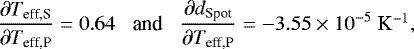
In Table 3, we also provide a statistical error estimate, derived from a Markov chain Monte Carlo (MCMC) analysis of the posterior probability distribution. The uncertainties are approximated by the standard deviation of the respective marginal distribution. We caution, however, that the posterior and therefore these uncertainties are all conditional on the assumptions, such as that of large, circular spots on the equator. This is most obvious in an uncertainty of 0.1 K for Teff,S, which obviously hinges on the fixing of Teff,P. To study the dependence of the system parameters on the assumed primary effective temperature, we repeat the modeling with values between 5000 and 7000 K. The only parameters strongly affected are the effective temperature of the secondary and the spot-dimming factor. In the considered range, the change in these parameters is well reproduced by linear relations for which we find slopes of
 (4)
(4)
where dSpot is the spot dimming factor. The inherent uncertainty in Teff,P therefore does not severely impede our ability to determine the system geometry. Nonetheless, systematic uncertainties likely also affect other parameters such as the mass ratio, q, which is notoriously difficult to determine via light-curve modeling in detached binary stars (e.g., Wilson 1994). In the following, we use the here-obtained best-fit model to represent the binary light curve without starspot contributions in the following modeling.
Best-fit (minimum χ2) parameters for CoRoT 105895502 derived from the light curve analysis of epoch 47.
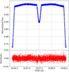 |
Fig. 7 Light curve (top panel) along with the residuals with respect to the best-fit model for epoch 47 (bottom panel). |
4.3 One- and two-spot models for all epochs
A model with a single starspot as introduced in Sect. 4.2 yields an acceptable fit for the particularly symmetric light curve of epoch 47. We now use a similar approach to model the light curve of all available epochs. Here we focus, however, on the starspot evolution and assume the light curve of the unspotted binary to be known. Specifically, we fix all parameters unrelated tothe spot properties to the best-fit values derived in Sect. 4.2. In the following modeling, we consider the fits to all individual epochs independent.
 |
Fig. 8 System geometry with primary (blue, left panel) and secondary (red, right panel) at orbital phase 0.44, i.e., shortly before secondary eclipse. Dotted arrows mark the model stellar rotation axes, which are assumed to be aligned with the orbit normal. |
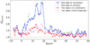 |
Fig. 9 Evolution of the reduced χ2 value as a function of epoch for the one-spot (blue circles) and two-spot models (red stars). |
4.3.1 One-spot modeling
In a first attempt, we fit the light curves of all individual epochs assuming a single starspot with a radius of 20° located on the equator of the secondary component. In the fit, the spot longitude and dimming factor as well as the model normalization are considered free parameters.
In Fig. 9, we show the temporal evolution of the resulting reduced χ2 value. Around epoch 47 the fit quality is optimal, which we attribute to the fact that the binary parameters were derived based on this epoch. Between about epoch 0 and 20, the fit quality of the one-spot model is worse than during the rest of the light curve; we postpone a more detailed discussion of this fact. We note that the fit quality is essentially identical if the spot is located on the primary instead of the secondary component (see Fig. 9).
In the top panel of Fig. 10, we show the evolution of spot longitude as a function of epoch. With the exception of the range between epochs 0 and 20, the time evolution of the spot longitude, lSpot, is well described by a linear model of the form
 (5)
(5)
where E is the epoch. According to our model, the spot shifts by about 5° per epoch or about 2.3° per day. With respect to the binary orbit, the spot advances in the direction of rotation, that is, its motion is prograde. Based on this relation, we estimate an uncertainty of about 4° for individual spot longitudes. The scatter is larger at the beginning until epoch 0, where the spot temperature contrast is also lower. During the observed time span, the model spot almost completes a revolution. Meanwhile, also its dimming evolves. The spot dimming increases most strongly until about epoch 20 after which further dimming appears to slow or eventually stop; we recall here, however, the worsened fit quality between epochs 0 and 20. Extrapolating the spot evolution into the domain prior to the start of the observation, we speculate that the spot emerged about ten epochs before the observation commenced. At any case, the spot lifetime is longer than the observational domain of 145 d.
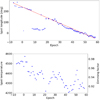 |
Fig. 10 Top panel: time evolution of spot longitude based on one-spot model along with an approximation to the observed trend (dashed red line). Symbol size is proportional to spot temperature contrast. Bottom panel: time evolution of spot temperature in model. |
4.3.2 Two-spot modeling
The fit quality of the one-spot model as shown in Fig. 9 is worst for the light curves of epochs 0 to 20, indicating that the model is insufficient to describe the data there. Therefore, we introduce a second spot in our modeling. As for the first spot, we fix the spot latitude and radius and only allow the longitude and dimming factor to vary. In order to avoid “spot collisions” in the modeling, we place this second spot on the primary component of the binary, which is not necessarily its physical location however. In the following, we refer to the spots as the primary and secondary spot depending on the component on which they reside.
In a first attempt at the two-spot model, we vary the longitudes and dimming factors of both spots along with the normalizing constant. The resulting fit quality is shown in Fig. 9 (red squares). Clearly, the fit quality for the light curves between epochs 0 and 20 improves substantially owing to the introduction of the primary spot, and expectedly the fit is not worsened otherwise. This justifies the introduction of the primary spot at least during the said epochs, for which a substantial improvement in the fit quality is obtained. Still, a small decrease in fit quality persists between epochs 0 and 20, which may be attributable to the presence of further spots or the limitations of our spot representation in the modeling.
The toppanel of Fig. 11 shows the time evolution of the longitudes of both spots, again encoding the dimming factor by symbol size and superimposing the linear trend derived from our previous one-spot modeling. Clearly, the structure observed in the one-spot modeling is recovered by the two-spot approach, even though the spots on the primary and secondary component occasionally exchange roles in the model. Before epoch 0, the linear longitudinal relation for the secondary spot is not recovered, which we attribute to cross-talk with the primary spot component and the comparably weak temperature contrast of the secondary spot there. During epochs 0 to 20, the primary spot remains at a longitude of about 30°, after which the model favors a spot at a longitude of about 200°. Here, however, the improvement in fit quality is much more moderate, meaning that introducing this component may not actually be justified.
Both our one- and two-spot models result in solutions showing a structure with a rather well-defined linear time evolution of longitude. We therefore set up a two-spot model in which we fix the longitude of the secondary spot according to Eq. (5) and vary only the longitude of its primary counterpart as well as both dimming factors and the normalization constant. The result is displayed in the bottom panel of Fig. 11. The resulting pattern is similar to that obtained without the longitude constraint and the fit quality is not much worse (Fig. 9).
Based on the latter model, we calculate the SQD for both spots. The result is shown in Fig. 12. The maximum SQD reached in our modeling is about 0.6%, that is, the spot properties are such that the quadrature flux of the system is diminished by 0.6%. While the secondary spot grows in influence before about epoch 10, after which the level is maintained, the primary spot shows a shorter lifetime. According to our modeling, it grows and decays between epochs 0 and 20, corresponding to a lifetime of about 40 d. The actual structure observed here may be a comparably short-lived active region. While the rate of growth appears to be similar for the primary and secondary spot, no decay is observed for the secondary spot. Again, the interpretation of a primary spot at an SQD of approximately 0.1% is not entirely clear. This component could represent a real spot or compensate inaccuracies in the modeling of the unspotted binary or starspot components.
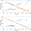 |
Fig. 11 Time evolution of spot longitudes in the two-spot model. The primary and secondary spots are indicated by orange circles and blue circles, respectively; an additional cross marks the secondary spot. Upper panel: model without longitudinal constraints. Evolution from one-spot model (Eq. (5)) as dashed, red line. Bottom panel: two-spot model with secondary spot longitude fixed according to Eq. (5). |
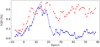 |
Fig. 12 Spot quadrature depression (SQD) for the two-spot model with fixed longitudinal time evolution for spot on secondary. Red points correspond to spot on secondary and blue squares to spot on primary. |
5 Discussion
We modeled the light curve of the eclipsing binary CoRoT 105895502 using the Nightfall code. First, we estimate the binary parameters by a fit to the light curve of a single epoch, which we identified as particularly well suited for that purpose. Secondly, we study the starspot evolution in the binary by modeling the CoRoT light curves of all available epochs. In this process, we fix the binary parameters and only adapt the starspot properties. In particular, we consider large spots with a fixed radius of 20°. While we adapt the longitude and temperature contrast of the spots via their dimming factor, the spots remain fixed at the stellar equator. In our modeling, we focus on models with one and two monolithic spots, which capture the effect of longitudinally asymmetric starspot surface concentrations such as active regions or longitudes on the light curve.
Both one- and two-spot models show the presence of at least one spot moving in prograde direction at a rate of about 2.3° per day. At the beginning of the observed light curve, our two-spot model shows the emergence of a new spot at a longitude of about 30°. This spot does not strongly move in longitude. Its effect is significant for at least 20 epochs or 40 days. In our modeling, its contribution fades at about epoch 25, after which the model favors a contribution from a spot at a higher longitude of about 200°. We caution here that some impact of this spot might be absorbed in the model of the spot moving in prograde direction, which approaches in longitude. Also, the improvement in fit quality obtained by introducing a second spot is rather moderate after epoch 20.
It appears that the lifetime of the spot associated with the prograde motion is longer than the observed span of 145 d. Prograde spot motion has been observed by Heckert & Ordway (1995), for example, in SS Boo, however on a longer timescale. In a study of light curves of short-term binaries observed with Kepler, Balaji et al. (2015) found spots moving in prograde direction in 13% of the studied systems. However, the major fraction of their binary sample show periods shorter than 2 days. In the short-period (≈ 0.5 d) eclipsing binary Kepler 11560447, Özavcı et al. (2018) find prograde shifts of active regions in the K1IV primary component of that system. The authors derive a rate of shift of 2.4° per day, which is quite compatible with our result.
Different hypotheses can be invoked to explain the presence of two spots, one moving in prograde direction and one with a rather constant longitude, between epochs 0 and 20 (see, e.g., Balaji et al. 2015). First, the spot moving in prograde direction may be located on a binary component, whose rotation is not synchronized with the binary orbit. In this scenario, the other spot would have to be located on the other binary component, whose rotation would have to be synchronized. The stellar rotation period of the component harboring the spot moving in prograde direction would then have to be shorter than the orbital binary period by about 1.4% or 0.03 d. Second, the relative spot motion may be a result of differential rotation. Assuming that both spots are really located on the same star, we can obtain an estimate of the strength of differential rotation on that star. By making the extreme assumption that one spot is located at the equator and one at the pole, we can derive a lower limit for the absolute value of the “relative horizontal shear”,
 (6)
(6)
on that star (e.g., Nagel et al. 2016). This yields a lower limit of 0.014 for α or 0.04 rad per day for the absolute horizontal shear. Clearly, the required latitudinal shear in rotation velocity must be larger to produce the same effect if the spots are closer in latitude. Also the sign of the shear remains unknown because we are ignorant of the order of spot latitudes. The resulting shear is consistent with the distribution of relative horizontal shear parameters derived by Reinhold et al. (2013) based on period analyses of a large sample of Kepler light curves. In this scenario, the rotationof at least some latitude of the stellar surface has to be synchronized with the binary orbit. In a third, alternative scenario, the observed behavior is caused by spot evolution, for example as a result of some sort of systematic evolution in the stellar magnetic field, resulting from an azimuthal dynamo wave for instance; this explanation was considered by Özavcı et al. (2018) for the case of Kepler 11560447. Whether the small eccentricity in the system plays a role in any of these scenarios can only be studied in a larger sample of systems. While we cannot distinguish between the scenarios based on the current analysis, it shows the potential of the ever-growing number of high-quality light curves of eclipsing binary stars for research on cool stars and stellar activity.
Acknowledgements
This work is based on data from the COROT Archive at CAB. This research has made use of the ExoDat Database, operated at LAM-OAMP, Marseille, France, on behalf of the CoRoT/Exoplanet program. S.C. acknowledges support through DFG projects SCH 1382/2-1 and SCHM 1032/66-1.
References
- Auvergne, M., Bodin, P., Boisnard, L., et al. 2009, A&A, 506, 411 [NASA ADS] [CrossRef] [EDP Sciences] [Google Scholar]
- Balaji, B., Croll, B., Levine, A. M., & Rappaport, S. 2015, MNRAS, 448, 429 [NASA ADS] [CrossRef] [Google Scholar]
- Bogdan, T. J., Gilman, P. A., Lerche, I., & Howard, R. 1988, ApJ, 327, 451 [NASA ADS] [CrossRef] [Google Scholar]
- Bradley, J. 1968, Distribution-free Statistical Tests (Englewood Cliffs, NJ: Prentice-Hall) [Google Scholar]
- Claret, A. 2000a, A&A, 359, 289 [NASA ADS] [Google Scholar]
- Claret, A. 2000b, A&A, 363, 1081 [NASA ADS] [Google Scholar]
- Czesla, S., Molle, T., & Schmitt, J. H. M. M. 2018, A&A, 609, A39 [NASA ADS] [CrossRef] [EDP Sciences] [Google Scholar]
- Deleuil, M., Meunier, J. C., Moutou, C., et al. 2009, AJ, 138, 649 [NASA ADS] [CrossRef] [Google Scholar]
- Djurašević, G. 1992, Ap&SS, 196, 241 [NASA ADS] [CrossRef] [Google Scholar]
- Efron, B., & Stein, C. 1981, Ann. Stat., 9, 586 [CrossRef] [MathSciNet] [Google Scholar]
- Gaia Collaboration (Prusti, T., et al.) 2016, A&A, 595, A1 [NASA ADS] [CrossRef] [EDP Sciences] [Google Scholar]
- Gaia Collaboration (Brown, A. G. A., et al.) 2018, A&A, 616, A1 [NASA ADS] [CrossRef] [EDP Sciences] [Google Scholar]
- Hauschildt, P. H., & Baron, E. 1999, J. Comput. Appl. Math., 109, 41 [NASA ADS] [CrossRef] [Google Scholar]
- Hauschildt, P. H., Allard, F., Baron, E., Aufdenberg, J., & Schweitzer, A. 2003 in Gaia Spectroscopy: Science and Technology, ed. U. Munari, ASP Conf. Ser. 298, 179 [NASA ADS] [Google Scholar]
- Heckert, P. A., & Ordway, J. I. 1995, AJ, 109, 2169 [NASA ADS] [CrossRef] [Google Scholar]
- Hendry, P. D., & Mochnacki, S. W. 1992, ApJ, 388, 603 [NASA ADS] [CrossRef] [Google Scholar]
- Huber, K. F., Czesla, S., Wolter, U., & Schmitt, J. H. M. M. 2010, A&A, 514, A39 [NASA ADS] [CrossRef] [EDP Sciences] [Google Scholar]
- Jeffers, S. V. 2005, MNRAS, 359, 729 [NASA ADS] [CrossRef] [Google Scholar]
- Kabath, P., Fruth, T., Rauer, H., et al. 2009, AJ, 137, 3911 [NASA ADS] [CrossRef] [Google Scholar]
- Kaplan, D. L. 2010, ApJ, 717, L108 [NASA ADS] [CrossRef] [Google Scholar]
- Kővári, Z., Oláh, K., Kriskovics, L., et al. 2017, Astron. Nachr., 338, 903 [Google Scholar]
- Kjurkchieva, D., Atanasova, T., & Dimitrov, D. 2016, Astron. Nachr., 337, 640 [NASA ADS] [CrossRef] [Google Scholar]
- Marilli, E., Frasca, A., Covino, E., et al. 2007, A&A, 463, 1081 [NASA ADS] [CrossRef] [EDP Sciences] [Google Scholar]
- Matson, R. A., Gies, D. R., Guo, Z., & Orosz, J. A. 2016, AJ, 151, 139 [NASA ADS] [CrossRef] [Google Scholar]
- Mazeh, T. 2008, EAS Pub. Ser., 29, 1 [Google Scholar]
- Meibom, S., Mathieu, R. D., & Stassun, K. G. 2006, ApJ, 653, 621 [NASA ADS] [CrossRef] [Google Scholar]
- Nagel, E., Czesla, S., & Schmitt, J. H. M. M. 2016, A&A, 590, A47 [NASA ADS] [CrossRef] [EDP Sciences] [Google Scholar]
- Özavcı, I., Şenavcı, H. V., Işık, E., et al. 2018, MNRAS, 474, 5534 [NASA ADS] [CrossRef] [Google Scholar]
- Parsons, S. G., Gänsicke, B. T., Marsh, T. R., et al. 2018, MNRAS, 481, 1083 [NASA ADS] [CrossRef] [Google Scholar]
- Pecaut, M. J.,& Mamajek, E. E. 2013, ApJS, 208, 9 [NASA ADS] [CrossRef] [Google Scholar]
- Pizzolato, N., Maggio, A., Micela, G., Sciortino, S., & Ventura, P. 2003, A&A, 397, 147 [NASA ADS] [CrossRef] [EDP Sciences] [Google Scholar]
- Raghavan, D., McAlister, H. A., Henry, T. J., et al. 2010, ApJS, 190, 1 [NASA ADS] [CrossRef] [EDP Sciences] [Google Scholar]
- Reinhold, T., Reiners, A., & Basri, G. 2013, A&A, 560, A4 [NASA ADS] [CrossRef] [EDP Sciences] [Google Scholar]
- Ribas, I. 2006, Ap&SS, 304, 89 [NASA ADS] [CrossRef] [Google Scholar]
- Santos, A. R. G., Cunha, M. S., Avelino, P. P., García, R. A., & Mathur, S. 2017, A&A, 599, A1 [CrossRef] [EDP Sciences] [Google Scholar]
- Siviero, A., Dallaporta, S., & Munari, U. 2006, Balt. Astron., 15, 387 [NASA ADS] [Google Scholar]
- Strassmeier, K. G. 2009, A&ARv, 17, 251 [NASA ADS] [CrossRef] [Google Scholar]
- van Kerkwijk, M. H., Rappaport, S. A., Breton, R. P., et al. 2010, ApJ, 715, 51 [NASA ADS] [CrossRef] [Google Scholar]
- von Zeipel, H. 1924, MNRAS, 84, 665 [NASA ADS] [CrossRef] [Google Scholar]
- Wald, A., & Wolfowitz, J. 1940, Ann. Math. Statist., 11, 147 [CrossRef] [Google Scholar]
- Wilson, R. E. 1994, PASP, 106, 921 [NASA ADS] [CrossRef] [Google Scholar]
- Yuan, H., Liu,X., Xiang, M., et al. 2015, ApJ, 799, 135 [NASA ADS] [CrossRef] [Google Scholar]
- Zahn, J. P., & Bouchet, L. 1989, A&A, 223, 112 [NASA ADS] [Google Scholar]
All Tables
Best-fit (minimum χ2) parameters for CoRoT 105895502 derived from the light curve analysis of epoch 47.
All Figures
|
Fig. 1 Revised white light curve of CoRoT 105895502. |
| In the text | |
|
Fig. 2 Excerpt of the light curve around a jump before correction (red, dashed) and the jump-corrected light curve (blue, solid) after flux level adjustment and removal of likely affected data points. |
| In the text | |
|
Fig. 3 Residuals of estimated eclipse times with respect to linear ephemeris for primary (blue dots) and secondary (red triangles) eclipses. Green crosses indicate the residuals of the secondary eclipse times with respect to the ephemeris derived from the primary eclipse timing. |
| In the text | |
|
Fig. 4 The S/N as a function of epoch. |
| In the text | |
|
Fig. 5 The asymmetry coefficient as a function of epoch. |
| In the text | |
|
Fig. 6 Convention of stellar longitude used in Nightfall. |
| In the text | |
|
Fig. 7 Light curve (top panel) along with the residuals with respect to the best-fit model for epoch 47 (bottom panel). |
| In the text | |
|
Fig. 8 System geometry with primary (blue, left panel) and secondary (red, right panel) at orbital phase 0.44, i.e., shortly before secondary eclipse. Dotted arrows mark the model stellar rotation axes, which are assumed to be aligned with the orbit normal. |
| In the text | |
|
Fig. 9 Evolution of the reduced χ2 value as a function of epoch for the one-spot (blue circles) and two-spot models (red stars). |
| In the text | |
|
Fig. 10 Top panel: time evolution of spot longitude based on one-spot model along with an approximation to the observed trend (dashed red line). Symbol size is proportional to spot temperature contrast. Bottom panel: time evolution of spot temperature in model. |
| In the text | |
|
Fig. 11 Time evolution of spot longitudes in the two-spot model. The primary and secondary spots are indicated by orange circles and blue circles, respectively; an additional cross marks the secondary spot. Upper panel: model without longitudinal constraints. Evolution from one-spot model (Eq. (5)) as dashed, red line. Bottom panel: two-spot model with secondary spot longitude fixed according to Eq. (5). |
| In the text | |
|
Fig. 12 Spot quadrature depression (SQD) for the two-spot model with fixed longitudinal time evolution for spot on secondary. Red points correspond to spot on secondary and blue squares to spot on primary. |
| In the text | |
Current usage metrics show cumulative count of Article Views (full-text article views including HTML views, PDF and ePub downloads, according to the available data) and Abstracts Views on Vision4Press platform.
Data correspond to usage on the plateform after 2015. The current usage metrics is available 48-96 hours after online publication and is updated daily on week days.
Initial download of the metrics may take a while.