| Issue |
A&A
Volume 627, July 2019
|
|
|---|---|---|
| Article Number | A25 | |
| Number of page(s) | 18 | |
| Section | The Sun | |
| DOI | https://doi.org/10.1051/0004-6361/201834154 | |
| Published online | 26 June 2019 | |
Two-fluid simulations of waves in the solar chromosphere
I. Numerical code verification
1
Instituto de Astrofísica de Canarias, 38205 La Laguna, Tenerife, Spain
e-mail: bpopescu@iac.es
2
Departamento de Astrofísica, Universidad de La Laguna, 38205 La Laguna, Tenerife, Spain
3
National Science Foundation, Alexandria, VA 22306, USA
Received:
29
August
2018
Accepted:
7
May
2019
Solar chromosphere consists of a partially ionized plasma, which makes modeling the solar chromosphere a particularly challenging numerical task. Here we numerically model chromospheric waves using a two-fluid approach with a newly developed numerical code. The code solves two-fluid equations of conservation of mass, momentum, and energy, together with the induction equation for the case of the purely hydrogen plasma with collisional coupling between the charged and neutral fluid components. The implementation of a semi-implicit algorithm allows us to overcome the numerical stability constraints due to the stiff collisional terms. We test the code against analytical solutions of acoustic and Alfvén wave propagation in uniform medium in several regimes of collisional coupling. The results of our simulations are consistent with the analytical estimates, and with other results described in the literature. In the limit of a large collisional frequency, the waves propagate with a common speed of a single fluid. In the other limit of a vanishingly small collisional frequency, the Alfvén waves propagate with an Alfvén speed of the charged fluid only, while the perturbation in neutral fluid is very small. The acoustic waves in these limits propagate with the sound speed corresponding to either the charges or the neutrals, while the perturbation in the other fluid component is negligible. Otherwise, when the collision frequency is similar to the real part of the wave frequency, the interaction between charges and neutrals through momentum-transfer collisions cause alterations of the waves frequencies and damping of the wave amplitudes.
Key words: Sun: chromosphere / Sun: oscillations / Sun: magnetic fields / methods: numerical
© ESO 2019
1. Introduction
Solar chromosphere is a transition layer where the properties of plasma change abruptly from being dominated by gas pressure (as in the photosphere) to being dominated by magnetic field (in corona), and where the collisional coupling of the plasma weakens with height. Several aspects of chromospheric physics make this region one of the most complex for understanding of the solar atmosphere.
It is well known that the chromosphere is not in local thermodynamic equilibrium (LTE). Athay & House (1962) measured and compared intensities in strong emission lines of H, He I, He II, and Ca II, and the deduced ratios of the populations of various levels indicated a significant departure from a Boltzmann distribution of the levels studied. In the high chromosphere the ratio of neutral atoms to ions exceeds the LTE values by about 107–108 in the case of He I and by about 106–107 in the case of hydrogen, and there is evidence that significant departures from LTE extend well into the photospheric layers. The formation of many photospheric lines is well described using LTE when radiation is fully coupled to the local physical conditions. However, in the chromosphere when collisional rates are lower, the radiation begins to decouple from the local physical conditions, invalidating the LTE assumption.
Plasma in the chromosphere is only partially ionized. As the density decreases with height, the collision frequencies between different particle species decrease and the magnetic field begins to dominate the dynamics. The neutral species do not feel the magnetic field directly and this causes a partial decoupling between charges and neutrals when the collisional timescales between ionized and neutral atomic species become equal to or larger than the magnetohydrodynamic (MHD) timescales. Therefore, the classical MHD approach is not the best approximation to treat the plasma processes in the chromosphere. While realistic photospheric models based on the MHD approximation provide results that are practically indistinguishable from observations even in strongly magnetized regions (e.g., Rempel et al. 2009), this is not the case for the chromosphere (see e.g., the discussion in Leenaarts 2010). This is because observations do not reach scales where ion-neutral effects can be detected directly in plasma dynamics (see e.g., Fig. 1 in Khomenko et al. 2014) in the photosphere. However, in the chromosphere, these scales become larger and may be reached in some dedicated observations. Indirect ion-neutral decoupling effects such as heating are also more pronounced in the chromosphere (e.g., see Ni et al. 2018).
A suitable alternative to the MHD approach is a two-fluid plasma–neutrals model, numerically implemented in this work. This kind of model is most appropriate for high-density plasmas such as in the chromosphere, where kinetic models cannot be efficiently applied. Kinetic models have been successfully applied to the corona and the solar wind, where much lower particle density makes the problem more computationally feasible and the kinetic description more necessary and appropriate. Multi-fluid models preserve a number of important physical effects coming from weak collisional coupling, still allowing for an efficient implementation, as in any fluid-based description. While the motivation for multi-fluid modeling comes mainly from theoretical considerations, in recent years there have been attempts at direct observational detection of multi-fluid effects in the solar plasma through measurements of differences in ion and neutral velocities caused by loss of collisional coupling. By measuring the Doppler shift in ion Fe II and neutral Fe I lines simultaneously over the same volume of plasma, differences between ion and neutral velocities of the Evershed flow have been found by Khomenko et al. (2015) in sunspot penumbra as deep as the photosphere. Similarly, Khomenko et al. (2016) showed that non-negligible differences in He I and Ca II velocities exist in solar prominences when observed with sufficiently high cadence. While the measured neutral and ion velocities were the same in most of the spatial locations most of the time, they were observed to decouple in the presence of strong spatial and temporal gradients, such as wave fronts. However, Anan et al. (2017) concluded that the observed small differences in velocities of H I 397 nm, H I 434 nm, Ca II 397 nm, and Ca II 854 were indications of motion of different components in the prominence along the line of sight, rather than indications of decoupling. Direct detection of the decoupling effects would require the highest spatial and temporal resolution, apart from a careful selection of spectral lines for the analysis. More observational studies in the future will be needed to confirm or discard the detection of the decoupling effects.
Nevertheless, there exist other indirect indications of decoupling such as the those observed by Gilbert et al. (2007). These authors compared He I 1083 nm and Hα data in multiple solar prominences in different phases of their lifecycle, and were able to detect the drainage effects across prominence magnetic field with different timescales for helium and hydrogen atoms. Such drainage was predicted earlier by Gilbert et al. (2002) from simplified semi-analytical calculations. Further indirect evidence of ion-neutral decoupling was reported by de la Cruz Rodríguez & Socas-Navarro (2011) who deduced misalignment in the visible direction of chromospheric fibrils and measured the magnetic field vector. These latter authors noted that most of the fibrils aligned with the magnetic field, although there are a few noteworthy cases where significant misalignments occur, well beyond the observational uncertainty.
Misalignment of chromospheric fibrils and magnetic field was confirmed by Martínez-Sykora et al. (2016) by using advanced radiative MHD simulations, which included the effects of ion-neutral interactions in the single-fluid approximation (via ambipolar diffusion). It was shown that the magnetic field is indeed often not well aligned with chromospheric features. The misalignment occurs where the ambipolar diffusion is large, that is, ion and neutral populations decouple as the ion-neutral collision frequency drops, allowing the field to slip through the neutral population. The conditions for misalignment also require currents perpendicular to the field to be strong, and thermodynamic timescales to be longer than or similar to those of ambipolar diffusion.
The vast majority of studies of ion-neutral effects in solar plasmas address propagation of different types of waves and the development of instabilities in chromospheric and prominence plasma conditions. Zaqarashvili et al. (2011b) and Soler et al. (2013a) performed theoretical studies of the propagation of Alfvén waves in a uniform medium composed of protons and hydrogen atoms which interact by collisions. Refinements of this theory were introduced by Zaqarashvili et al. (2011a) by adding helium atoms, by Zaqarashvili et al. (2013) by considering a nonuniform gravitationally stratified atmosphere, and by Soler et al. (2013b) by applying a flux tube model. It was found that in situations when the neutral-ion collisional frequency is much lower than the wave frequency, the propagation properties of the waves only depend on the properties of the ionized fluid. These properties change with height due to stratification, and the Alfvén wave may become evanescent in some regions of the solar atmosphere. The waves can be damped by neutral-ion collisions, and the existence of neutral helium atoms, alongside with neutral hydrogen, significantly enhances the damping. The damping is most efficient when the wave frequency and the collisional frequency are of the same order of magnitude. The overall conclusion from these studies is that the single-fluid approach is suitable for dealing with slow processes in partially ionized plasmas, which happen on longer timescales than the collisional timescale. This approximation fails for timescales comparable to or shorter than the characteristic timescales for interaction between the charged and neutral particle populations.
Only recently, several numerical simulations of solar phenomena using a two-fluid approach have been reported. However, their realism is rather limited. Maneva et al. (2017) modeled magneto-acoustic wave propagation in the solar stratified chromosphere including effects of impact ionization and radiative recombination. These authors found numerous difficulties in constructing an equilibrium model atmosphere for the wave propagation, and in interpreting the results of their simulations in comparisons to more standard, single-fluid models. Magnetic reconnection has been studied using a two-fluid model by Smith & Sakai (2008), Leake et al. (2012, 2013), Alvarez Laguna et al. (2014), and Hillier et al. (2016). Important decoupling between the flows of neutrals and ions was observed in their simulations close to a reconnection site with considerable differences between inflows and outflows. Ni et al. (2018) also found that even in the absence of flow decoupling, dynamics of the ionization and recombination processes can have important consequences for the thermodynamics and observable properties of plasma at chromospheric reconnection sites. Martínez-Gomez et al. (2017) used a five-fluid model with three ionized and two neutral components, which takes into consideration Hall current and Ohm’s diffusion in addition to the friction due to collisions between different species. These latter authors apply their model to study the wave propagation in homogeneous plasmas composed of hydrogen and helium, similar to analytical models described above, but allowing time evolution of the ionization fraction. They confirmed the theoretical result that the inclusion of neutral components in the plasma modifies the oscillation periods of the low-frequency Alfvén waves and that collisions produce damping of the perturbations, the damping being more efficient when the collisional frequency is of the order of the oscillation frequency.
Considering all of the above it is evident that numerical modeling of solar chromospheric plasma including multi-fluid effects is a promising approach, and that a significant effort is required in this direction. Both previous theoretical and observational results suggest the need for such modeling. Here, we describe the results from the newly developed two-fluid code for purely hydrogen plasma which takes into account the effects of elastic and inelastic interactions between electrons, ions, and neutral atoms. In the current paper, which is the first in our study of chromospheric waves and shocks within a multi-fluid approximation, we verify the code against known analytical solutions for the wave propagation in a homogeneous plasma, and provide numerical convergence results of the implemented numerical scheme. In Sect. 5 we describe a test of a fast wave in a gravitationally stratified atmosphere, and test the numerical solution against the analytical solution. The full equations are provided in this first paper, describing the upgraded code, in order to enable reproducibility, and for future reference in the follow-on papers. In the second paper of the series (Popescu Braileanu et al. 2019), we apply the code to study the nonlinear behavior of chromospheric shocks under two-fluid conditions.
2. Numerical method
A multicomponent plasma evolution can be described by equations of continuity, momentum, and energy of its components which are obtained via momenta (0th, 1st, and 2nd moment) of the Boltzman equation. Typically, ions(i), electrons(e), and neutrals(n) are considered. When treated numerically with an explicit code, the equation of evolution of electrons imposes very small time steps and is therefore numerically restrictive. Because of the large ion-to-electron mass ratio, the electron propagation speed, sound speed, and Alfven velocity are also large relative to the corresponding bulk plasma parameters; this restricts the time step in an explicit scheme. However, for the same reason, the electron mass effects can generally be neglected from the electron equation of motion. This relaxes some of the numerical constraints and results in a generalized Ohm’s law used to compute the evolution of the electric field. The following assumptions are made in the set of two-fluid equations implemented in this work:
-
Purely hydrogen plasma. This condition implies than only singly ionized ions are present and that charge neutrality is fulfilled on scales above the Debye radius scale, as usual. Charge exchange reactions are introduced via elastic collisions, by defining a charge-exchange collisional parameter αcx, added to the elastic collisional parameter α. The expression of this term is given in Eq. (A.5). For such plasma, a constant mean molecular weight for neutrals is μn = 1 g mol−1 and a constant mean molecular weight for charges is μc = 0.5 g mol−1, where the sub-index “c” stands for “charges”.
-
Identical temperatures of ions and electrons, that is, Tc = Te = Ti. Neutrals and charges are allowed to have different temperatures, that is, generally Tn ≠ Tc.
-
The center of mass velocity of charges is essentially ion velocity, that is, uc = ui. This condition implies that
 .
.
2.1. Equations
We solve continuity, momentum, and energy conservation equations written separately for charges (sub-index “c”) and neutrals (sub-index “n”). The interaction between neutrals and charges is introduced via the different kinds of collisional terms, as follows.
2.1.1. Continuity equations
with:
the latter being the ionization/recombination collisional source term. The variables Γion and Γrec are ionization and recombination rates and are defined in Appendix A. The variables ρc and ρn are mass density of charges and neutrals, and uc and un are their center of mass velocities.
2.1.2. Momentum equations
The elastic collisions between ions and neutrals and between electrons and neutrals can be combined into a single collision frequency between charges and neutrals. By defining the collisional parameter:
the effective collision frequencies between charges and neutrals, and between neutrals and charges become, respectively:

Here, νen and νin are the electron-neutral and ion-neutral collision frequencies, respectively, with expressions given in Eq. (A.3). If we take into account the charge-exchange reactions, αcx, as defined in Eq. (A.5) should be added to the elastic collision parameter α. The momentum collisional term Rn can be written as

Here  and
and  are pressure tensors for charged and neutral species, B is magnetic field, J is current density, and Rn is momentum collisional exchange term. The latter takes into account momentum gains/losses due to elastic collisions, with collisional frequencies between ions, electrons, and neutrals, νin and νen, defined in Appendix A; it also takes into account momentum gains/losses due to ionization and recombination (the terms proportional to the ionization/recombination rates Γ).
We consider isotropic pressure, but we include viscosity in the pressure tensor:
where the elements of the viscosity tensor are
The expressions used for the viscosity coefficient for species α, denoted by the symbol ξα, are given in Eq. (A.10).
The gravitational acceleration g is oriented in the negative z direction.
2.1.3. Energy conservation equations
with:
In these equations, ec and en are charges and neutral internal energy, respectively, and Tc and Tn are the corresponding temperatures, Kc and Kn are thermal conductivity coefficients, whose expressions are shown in Eq. (A.10). Among the four terms of the expression of Mn, the first two are related to ionization/recombination processes, and the last two terms are related to elastic collisions. Terms containing temperatures, namely the second and the fourth terms, represent the thermal exchange between charges and neutrals due to inelastic and elastic collisions, respectively. Because the energy equations evolve kinetic and internal energy, the Mn terms include kinetic energy gains/losses due to the change in the number of particles, and to the work done by the collisional terms. One can write equations of evolution of internal energy alone:
where
is the nonideal part of the electric field E, and
which is the heating due to the viscosity, is a non-negative quantity. Subsequently, the collisional terms become, for neutrals and charges:
We observe that the second and the fourth terms remain unchanged. However, the first and the third terms are different; they become non-negative quantities and thus contribute to dissipative heating. The neutrals and charges are heated because of recombination and ionization processes, respectively (the first term), and both species are heated at the same rate by elastic collisions (the third term, equal for neutrals and charges, also called “frictional heating”). Most expressions of the terms related to collisions (including coefficients of viscosities, thermal conductions, and magnetic resistivity) are derived by Braginskii (1965), but they are also detailed in the descriptions of models by Meier & Shumlak (2012), Leake et al. (2012, 2013).
The relation between internal energy and pressure, and between the pressure, the number density, and the temperature are defined by ideal gas laws:
2.1.4. Ohm’s law
In order to obtain Ohm’s law we operate on the momentum equation for ions and electrons. For the case of purely hydrogen plasma, and by neglecting terms proportional to me/mi, such as electron inertia terms, and time variation of currents (see Khomenko et al. 2014; Ballester et al. 2018), we obtain to the following expression.

where
All four terms on the right-hand side of Eq. (14) are the same as in the single fluid approach, and the first three of them represent the Hall term, the Biermann battery term, and the Ohmic term. The fourth term, proportional to the difference of the velocities of the two species, is usually neglected in both approximations. The ambipolar term, which appears in the single-fluid approximation as a consequence of the charged and neutral fluids having different center-of-mass velocities does not appear in the two-fluid approach. The derivation of these terms can be found in Khomenko et al. (2014).
The induction equation for the evolution of the magnetic field is obtained using Maxwell equations, in a usual way,
2.2. Numerical implementation
2.2.1. MANCHA3D code
In this work we have extended the MANCHA3D code, a single-fluid code, where the effects of partial ionization have been implemented through a generalized Ohm’s law including Ohmic, ambipolar, and Hall and Biermann battery terms. The new code solves the two-fluid equations in approximation of purely hydrogen plasma, as described above. Ions and electrons are evolved together through the same continuity, momentum, and energy equations, and neutrals are evolved separately. The neutral and charges equations are coupled by collisions. These new developments are described below.
The original MANCHA3D code is described elsewhere (Khomenko & Collados 2006, 2012; Felipe et al. 2010; González-Morales et al. 2018). The code is fully 3D, written in Fortran 90, and parallelized with MPI; the output files are in HDF5 format. The units used in the equations are SI units. The variables are split into background and perturbation variables, keeping all nonlinear terms. The viscous forces and the Ohmic dissipation tend to eliminate high-frequency oscillations. However, collisional viscosity (ξc, n; Eq. (8)) and Ohmic (ν; Eq. (14)) coefficients for the parameters of the solar atmosphere are too small to effectively damp nonresolved variations of different parameters at the grid cell size. Therefore, for numerical stability, these coefficients have corresponding numerical analogs referred to as hyperdiffusive coefficients. The hyperdiffusive coefficients correspond to physical terms: magnetic Ohmic diffusion, conductivity, viscosity, and so on. The amplitude of the hyperdiffusive coefficients is a complex function of space coordinates and of gradients of the corresponding variables (for details see Vögler et al. 2005; Felipe et al. 2010). Since high numerical diffusion is not always desirable, an additional filtering of small wavelengths following Parchevsky & Kosovichev (2007) is implemented in MANCHA3D. In order to avoid reflections at the boundaries, MANCHA3D uses the Perfect Matching Layer technique (Felipe et al. 2010). The spatial discretization scheme is fourth-order accurate. The original temporal discretization scheme was a fourth-order explicit Runge–Kutta, modified to an arbitrary order in the latest version of the code due to implementation of STS and HDS schemes (González-Morales et al. 2018). The two-fluid implementation required further modification of the explicit Runge–Kutta integration. The new implementation is a semi-implicit scheme with up to second-order accuracy, as is shown in the numerical tests of the code described below.
2.2.2. Numerical scheme
Since the solar atmosphere is strongly gravitationally stratified, the collisional frequencies change orders of magnitude from the photosphere to the chromosphere. In the deep layers, collisional terms are typically very large and dominate over the hydrodynamical timescales. In the chromosphere this situation may change, since collisional frequencies become significantly smaller. Therefore, the numerical scheme of our two-fluid numerical code has to be able to handle large variations in collision frequencies. In the case of dominant collisional terms the equations become stiff and therefore an explicit integration scheme is unstable. This is because the collisional terms that appear in the equations of continuity, momentum, and energy are proportional to the collision frequency, and the time step should be at most the inverse of the collision frequency in order to ensure stability in an explicit scheme. This imposes very small time steps when the collisions are dominant. A suitable alternative is to use semi-implicit schemes similar to that described by Toth et al. (2012), such as the one implemented here. Our system of equations, Eqs. (1), (3), (9), and (14), can be schematically written as follows.

where U is the vector of variables,
and R(U) is the sum of fluxes and collisional terms.
In order to evolve this system of equations in time: we split R into an explicit operator E and an implicit operator P,

The explicit operator E(U) contains fluxes, while the implicit operator contains the collisional terms, Eqs. (2), (6), and (10). With U* being the solution after applying the explicit update,
we apply the implicit update using the following discretization.

The value of β can vary between 0 and 1, and its influence on the final solution will be discussed below.
The code solves three systems of two coupled equations during the implicit update, with U being in the three cases a vector with two components, as defined above by Eq. (18),  , meaning that all of the collisional terms, namely Sn, Rn, and Mn defined in Eqs. (2), (6), and (10), can be treated in the same way. We note however that depending on the magnitude of the collisional terms Sn in the continuity equations, it might not be worth treating them implicitly. In such cases we add these terms into the explicit operator E(U). All the terms on the right-hand side of the induction equation, Eq. (14), are treated explicitly.
We linearize P(Un + 1) around the value of U* after an explicit update:

where the Jacobian, Ĵ, is defined as follows.

Due to particular symmetry properties of the equations, J21 = −J11, J22 = −J12. This allows the solution for the implicit update to be calculated directly. The update in one sub-step of a two-step Runge–Kutta scheme can then be summarized as
where k = 2, 1;  is the time step used in the substep, and Δt is the complete time step. The scheme parameter
  can have a different value in each substep (subscript
  ). The magnitude of Δt is limited by the MHD CFL condition. The explicit operator, E, is recalculated in each Runge–Kutta sub-step using the variables updated after the previous sub-step. The Jacobian Ĵ is also calculated after the explicit update, so that Ĵ = Ĵ∗.
The elements of the Jacobian can be written in the analytical form.
For the momentum equations, this ensures that

For the energy equations, the same expression becomes
where Um and UT are the kinetic and internal energy parts of the variable U, respectively. The Ĵ and K̂ for the energy equation are defined as follows.
The variable  is the difference between U* after an explicit update, and one Runge–Kutta sub-step of the implicit update, i.e.,
Overall, this means that the energy implicit update is done with variables calculated after the momentum implicit update. The analytical expressions for Ĵ and K̂ are given in Appendix B. The numerical scheme is stable when we use the time step imposed by the CFL. For  and
and  the scheme is formally second-order accurate.
3. Analytical model of waves in a uniform plasma
Our newly implemented scheme has been checked using simulations of wave propagation in a uniform plasma. We used two simple analytical cases. In the first case we consider purely acoustic waves propagating in an atmosphere where the background equilibrium temperature of charges and neutrals is different. In this case the difference in behavior between charges and neutrals is created by the different sound speeds of the background atmosphere. In the second case we consider the propagation of Alfvén waves. Here the difference in the behavior of charges and neutrals is produced additionally due to the presence of the magnetic field. In this simple setup the problems have analytical solutions that can be obtained by linearizing the two fluid equations and looking for solutions in the form of monochromatic waves. The sections below describe the analytical solution and results for both sets of simulations, together with the tests of numerical convergence of the scheme.
3.1. Acoustic waves
Acoustic waves are longitudinal waves, therefore their velocity vector and direction of propagation are parallel, that is, un ∥ k and uc ∥ k. We choose the direction of propagation along z direction. We neglect the effects of ionization, recombination, thermal exchange, thermal conduction, and radiation. Therefore, we only consider the momentum exchange due to elastic collisions. In this simple situation the linearized continuity, momentum, and adiabatic energy equations become
where unz and ucz are the velocity projections along z direction, and cn0 and cc0 are sound speeds of neutrals and charges. Variables with subscript “0” refer to the background unperturbed atmosphere, and variables with subscript “1” refer to the perturbation. The collisional parameter α defined by Eq. (4) uses the values of the unperturbed mass densities of electrons, ions, neutrals, and charges. Since for the simple model assumed here the value of α only depends on the homogeneous background variables in the linear approximation, it is kept constant in time and space.
We search for solutions of form,

where {Un, Uc, Rn, Rc, Pn, Pc} are, in general, complex amplitudes for all the perturbed variables. These amplitudes are related through the so-called polarization relation, so one needs to set one of the amplitudes to obtain the rest of them through the following relations:
The resulting dispersion relation, which relates the frequency and the wavenumber, has the following form:
Once the background values are specified, the value of the collisional parameter α is determined. It is then convenient to operate in terms of the following parameters: ω/k, and α/k. The latter ratio is an effective measure of the collisional strength. The analysis below will be done in terms of the nondimensional variables:
These variables are similar to those used in Soler et al. (2013a). Later on in the paper we represent the solution of the dispersion relation in terms of these nondimensional variables, keeping in mind that F is inversely proportional to the wavenumber k with the mutiplicative factors fixed (by “varying the collisional strength F” we understand varying the wavenumber k, since the value of α is fixed).
Using nondimensional variables, the polarization relations and the dispersion relation become:

where:
Here ρtot = ρn0 + ρc0 and  are the total density and the sound speed of the whole fluid.
3.2. Alfvén waves
Alfvén waves are transverse incompressible waves, polarized perpendicularly to the direction of the background magnetic field. The analytical solution for the Alfvén wave propagation in partially ionized plasma used in our work is similar to those developed previously by Soler et al. (2013a). We consider here a simple case of Alfvén waves with propagation only along the background magnetic field. These are frequently called pure Alfvén waves. In our case, k ∥ B0, un ∥ B1, uc ∥ B1, B1 ⊥ B0. We choose the equilibrium magnetic field along z direction and perturbation of magnetic field and velocities along x direction.
Otherwise the assumptions of the equations are similar to the acoustic wave case. The linearized momentum and induction equations take the following form.
The equations of continuity and energy conservation are not needed in this case because the Alfvén waves are purely incompressible. Similar to acoustic waves we use the solutions of the form

where the amplitudes can be complex in general. Plugging this ansatz into Eq. (36), we obtain the following polarization relations.
and the dispersion relation in the following form.

For the same reason as for the acoustic waves, we vary the collision strength by varying the wavenumber k parameter to study its influence on the propagation properties of the waves. Using the nondimensional variables:
the dispersion relation, and the polarization relations are
3.3. Background atmosphere
The values of the uniform background atmosphere used in this study are given in Table 1. For the Alfvén wave tests, a z-directed magnetic field B0 = 5 × 10⁻³T is also added. The corresponding Alfvén speed calculated using the density of charges is  m s−1. The collisional parameter α defined in Eq. (4) calculated for the background has the value 7.324 × 10¹² m3 kg−1 s−1. In this test the temperature of electrons is assumed to be zero, they do not contribute to the pressure of charges, and the effective neutral-charge and charge-neutral collision frequencies defined in Eq. (5) become the neutral-ion and ion-neutral collision frequencies, with values νni ≈ 3.65 × 10⁴ s−1, and νin ≈ 7.3 × 10⁴ s−1, respectively.
Values of the background atmosphere parameters used in the tests of the wave propagation in the uniform medium for neutrals (left) and charges (right).
3.4. Parameters of the perturbation
We have to supply several free parameters to calculate the solution. We have chosen the real wave number k, and obtain the complex ω from the dispersion relations, Eqs. (31) and (39). This means that we consider wave damping in time. Additionally, since the perturbations in all the magnitudes are related, we need to supply the amplitude of one of them in order to calculate the others. Generally, since the polarization relations are complex, there will be the phase shift between oscillations of different quantities.
We have selected the wavenumber to be k = 2πn/Lz m−1, with n being an integer number. We vary the wavenumber k by varying the domain length Lz in order to have n = 11 (a random choice) for all the simulations.
For the acoustic waves we choose the amplitude of the perturbation in density of charges, Rc = 10−3ρc0, and for the Alfvén waves we choose the amplitude of the perturbation in velocity of charges, Uc = 10−5vA0. We calculate the other amplitudes from Eq. (30) for the acoustic waves and Eq. (36) for the Alfvén waves. In all cases, for the numerical solution we used periodic boundary conditions. For the initial condition of the perturbation we used the analytical solution at t = 0 s in the whole domain.
We run all simulations for a total time tF so that we have Lz/tF equal to 7447.273 m s−1 for all the simulations of acoustic waves and equal to 32125.49 m s−1 for the Alfvén wave simulations. These values are of the order of the characteristic speeds: the sound speed and the Alfvén speed.
3.5. Solution of the dispersion relation for acoustic waves
The acoustic wave dispersion relation is a fourth-order equation in both ω and k. If the neutrals and charges have the same background temperature, the dispersion relation has four solutions, with simple expressions as shown in Eq. (44). In our case Tc0/Tn0 = 4, and the values of the coefficients in Eq. (34) are a2 = 5/2 and a0 = 1, and the expressions for the solutions, obtained using Mathematica software, in this case are as follows.
We compute the complex frequency, ω, for the values of k between 6180 and 6.18 × 10⁻⁶ m−1, for each of the four expressions of the mathematical solutions shown in Eq. (43), and marked as solutions 1, 2, 3, and 4 in Fig. 1. The real and imaginary parts of the four solutions are shown in the normalized units, E = f(F), defined in Eq. (32), that is, ω{I, R}/k/ctot as a function of αρtot/k/ctot for better visualization. The solutions with positive ωR travel in the positive direction of the z axis, and those with negative ωR travel in the negative direction.
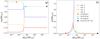 |
Fig. 1. Solutions of the dispersion relation, Eq. (31), for the acoustic wave case. Left and right panels present the real and imaginary parts of the dimensionless wave frequency ω, respectively, as functions of the dimensionless wavenumber k. The axes are scaled in nondimensional units E and F, defined in Eq. (32) for better visualization. Four solutions are marked with different colors and line styles: solid red for solution 1, orange dashed for solution 2, blue dot-dashed for solution 3, and green dotted for solution 4. We note that solutions 1 and 4 have the same imaginary parts and are superposed in the right-hand panel. Solutions 2 and 3 have the same real part equal to zero for large α/k and are also superimposed on top of one another. The values of k for which we compare the analytical and numerical solution using the values of ω, corresponding to solution 4 (green dots), are marked in the panels: orange circle (k = 618 m−1), pink triangle (k = 6.18 m−1), cyan diamond (k = 2.06 m−1), and black “X” (k = 6.18 × 10⁻⁶ m−1). |
Waves corresponding to solutions 1 and 4 (red and green colors) propagate with a speed (vph = ωR/k) equal to the sound speed of the charges ( ) for small ratios α/k, in the negative and positive direction of the z axis, respectively. For the large values of α/k, their propagation speed becomes that of the whole fluid, ctot. The imaginary part of the frequency ωI is positive meaning wave damping. The imaginary part would be zero if the charges and neutrals had the same background temperature, since in that case the solutions of the dispersion relation, Eq. (34), would simplify to

with zero imaginary part for solutions 1 and 4. As the only difference between neutrals and charges in this particular model is in their sound speed, it is not surprising that by making the sound speed the same the damping disappears, since both fluids would oscillate with exactly the same velocity and therefore the frictional damping term would become strictly zero.
The value of damping is the same for solutions 1 and 4. For either very low or very high values of the ratio α/k, the damping relative to the wavenumber (ωI/k) is small and approaching zero. The value of the ratio ωI/k is maximum at a point located on the x axis at  , and corresponds to kM ≈ 7.5 m−1. E(F = FM) =
  ; this gives the value of
  , which means that the real part of the wave frequency is approximately equal to the ion-neutral collision frequency at the point where the damping relative to wavenumber, the ratio ωI/k, is maximum (FM).
Waves corresponding to solutions 2 and 3 (yellow and blue colors) propagate with a speed equal to the sound speed of neutrals ( ) for small values of α/k. For large α/k, these solutions have zero propagation speed (zero ωR). The ratio ωI/k is again small for weak or strong collisional coupling (small or large α/k), and has the maximum located on the x axis at a point very close to FM.
These results are easy to interpret. For small collisional frequencies compared to the real part of the wave frequency, i.e., weak collisional coupling, the propagation of the waves mostly depends on the properties of either of the fluids. Since the neutrals and the charges have different sound speeds, in the case of weak collisional coupling the waves propagate either at the sound speed of neutrals or of charges. Correspondingly, if one perturbs charges with a certain amplitude, the weak drag forces will translate some of this perturbation to neutrals, but the amplitude of this perturbation will be very small, as indeed follows from the polarization relations in Eq. (30). The opposite is also true.
For large collision frequencies compared to the real part of the wave frequency, that is, strong collisional coupling, the charges and the neutrals become coupled and the wave propagates at the sound speed of the whole fluid. Subsequently, the amplitudes of the velocities of neutrals and charges are equal.
For the numerical tests, we only show the results corresponding to solution 4 (the green lines in Fig. 1), that is, the solution for waves which propagate at the sound speed of the charges for small α/k. The results in other cases are similar. We have selected one wavenumber so that αρtot/k/ctot is less than FM, and three values of k, for which this quantity is larger than FM. These frequencies are marked with symbols in Fig. 1. In order to relate the results to observations, Table 2 provides the period, P = 2π/ωR, and the damping time, TD = 2π/ωI for the waves used in the simulations (the wavenumbers k marked in Fig. 1), and for the wave corresponding to the maximum damping relative to the wavenumber (with wavenumber kM) in physical units. We can see that the waves have extremely short periods and wavelengths and do not correspond to the waves observed in the chromosphere, which have typical frequencies of 3–5 mHz. This is due primarily to our use of a uniform, unstratified background atmosphere which does not correspond to the chromosphere. The temperatures of charges and neutrals differ by a factor of four, and this situation is also unrealistic. For these reasons, the value of the collisional parameter α corresponding to the background atmosphere may be unphysical for the chromosphere. Moreover, for the purposes of code verification we wanted to test both uncoupled and strongly coupled cases, and the values of k that we have chosen cover the full range, even if the waves corresponding to the largest values of k have small temporal and spatial scales that cannot be observed.
Values of the period, and damping time for the acoustic waves.
3.6. Solution of the dispersion relation for Alfvén waves
As in the case of the acoustic waves, we solve the dispersion relation for values of k between 6180 and 6.18 × 10⁻⁶ m−1, and we plot the real and imaginary parts of the wave frequency in Fig. 2, as a function of the wavenumber in nondimensional units, C = f(D), defined in Eq. (40), i.e., ω{I, R}/k/vA0 as function of αρtot/k/vA0. The dispersion relation is a third-order equation in ω and there are three solutions. In our case, ρc0/ρtot = 1/3, and the solutions obtained using Mathematica software are
with

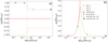 |
Fig. 2. Solutions of the dispersion relation, Eq. (39), for the Alfvén wave case. Left and right panels present the real and imaginary parts of the wave frequency ω, respectively, as a function of the wavenumber k. The axes are scaled in the nondimensional units: C and D, defined in Eq. (40) for better visualization. Three solutions are marked with different colors and line styles: red solid for solution 1, orange dashed for solution 2, and green dotted for solution 3. The values of k for which we compare the analytical and numerical solutions using the values of ω, corresponding to solution 3 (green dots), are marked in the panels: pink triangle (k = 61.8 m−1), green triangle (k = 6.18 m−1), orange star (k = 6.18 × 10⁻² m−1), and black triangle (k = 6.18 × 10⁻⁶ m−1). |
These represent one wave which does not propagate (ωR = 0, red color), one wave traveling in the positive direction of z axis (green color), and a similar wave traveling in the negative direction (yellow color).
For small values of the collisional frequency compared to the real part of the wave frequency, the propagation speed (vph = ωR/k) is the Alfvén speed considering only the density of charges (vA0). For the large values of α/k, the value of vph is the Alfvén speed of the whole plasma considering both neutrals and charges, vAtot. We note that  . With no collisions between charges and neutrals, the imaginary part of solutions 2 and 3 vanishes,

meaning that the damping is related to the presence of neutrals. In our case, the imaginary part is positive, and the maximum damping relative to the wavenumber, the ratio ωI/k, is located at a point  on the x axis, corresponding to a value of
  m−1. This gives the value of ωR(D = DM)/(αρn0) ≈ 1. As in the case of the acoustic waves, the real part of the wave frequency is almost equal to the ion-neutral collision frequency at the point where the damping relative to wavenumber is maximum. Otherwise, the damping relative to the wavenumber is very small.
For the numerical tests below we use the solution traveling in the positive direction of the z axis (green color in Fig. 2) and for values of the wavenumbers, k, indicated in the legend of Fig. 2. The period and the damping time for the waves used in the simulations (corresponding to the values of k marked in Fig. 2), and for the wave corresponding to the maximum damping relative to the wavenumber (with wavenumber  ) are given in Table 3. For the same reasons as the acoustic wave tests, the frequencies and the wavenumbers of the Alfvén waves do not correspond to typically observed waves in the chromosphere.
Values of the period, and damping time for the Alfvén waves.
4. Results of numerical calculations
We ran simulations of acoustic and Alfvén waves using the equilibrium atmosphere and perturbation described in Sects. 3.3 and 3.4 as initial conditions. We used several values of the wavenumber k marked in the corresponding panels described in the above section. In order to observe the damping in time we choose a point located in the center of the domain and plot the evolution of the variables at the same point as function of time. The numerical solution is then compared to the analytical solution.
4.1. Temporal damping of acoustic waves
Figure 3 shows the numerical and analytical solutions for the acoustic waves with wavenumber values of k = 618, 6.18, 2.06, and 6.18 × 10⁻⁶ m−1.
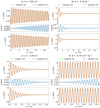 |
Fig. 3. Simulations of acoustic wave propagation in a homogeneous plasma. Numerically (red dashed line) and analytically (green solid line) calculated time evolution of the velocity of neutrals and charges as a function of time. Below the panels showing the velocity of neutrals, the difference (Δ) between the numerical solution and the analytical solution for unz is given. Time is measured in units of the wave period, 2π/ωR. Panels from left to right and from top to bottom: simulations for different values of the wavenumber k, as indicated in the legend of Fig. 1. |
We can observe that for different values of k the amplitude damping and propagation velocity vary in agreement with what is expected from Fig. 1. For the large value of k = 618 m−1 (panel a of Fig. 3) there is a phase shift between the oscillating fluid velocities of neutrals and charges, and both are slightly damped. We highlight the fact that the amplitude of oscillations of velocity of charges is significantly larger than that of the neutrals. For the intermediate values of k = 6.18 and 2.06 m−1 (panels b and c of Fig. 3), we observe significant damping of both velocity oscillations but similar amplitudes and a smaller phase shift. For the small k case, that is, k = 6.18 × 10⁻⁶ m−1 (panel d), the velocities of charges and neutrals are the same, and the wave propagation velocity is the sound speed of the plasma as a whole. This is expected since charges and neutrals are collisionally coupled.
We observe from Fig. 3 that numerical and analytical solutions are in very good agreement; in all panels, we plotted the difference between the numerical and the analytical solution, labeled Δ right below the plots for ucx. The error can be seen to accumulate over time, but this is nevertheless very small.
The values from Table 2 are consistent with the values deduced from Fig. 1. The amplitude of a wave will decrease to a fraction f = exp(−2πP/TD) in a period. For example, in the case of the wave with wavenumber k = 6.18 m−1, f ≈ exp(−9.6/7.37) ≈ 0.27, which is consistent with the value observed in panel b of Fig. 3.
4.2. Temporal damping of Alfvén waves
Figure 4 shows the numerical and analytical solutions for the Alfvén waves with the wavenumber k set to the following values, k = 61.8, 6.18, 6.18 × 10⁻², and 6.18 × 10⁻⁶ m−1. These values of k are marked in Fig. 2.
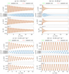 |
Fig. 4. Simulations of Alfvén wave propagation in a homogeneous plasma. Here we show the numerically (red dashed line) and analytically (green solid line) calculated time evolution of the velocity of neutrals and charges, and the magnetic field perturbation, as a function of time. Below the panels showing the velocity of charges, the difference (Δ) between the numerical solution and the analytical solution for ucx is plotted. Time is measured in units of the wave period, 2π/ωR. Panels from left to right and from top to bottom: simulations for different values of the wavenumber k, as indicated in the legend of Fig. 2. |
We observe that numerical and analytical solutions match exactly and the amplitude damping and wave propagation speed vary with the ratio α/k as expected from Fig. 2.
For small α/k, the wave propagates at the Alfvén speed of the charges and the velocity of neutrals is almost zero (panel a of Fig. 4). For large α/k, the wave propagates at the Alfvén speed of the whole fluid and the velocities of neutrals and charges are equal (panel d). Yet again, for intermediate values of α/k, the damping of all perturbations is observed (panels b and c).
For all the panels in Fig. 4, we show the difference between the numerical and the analytical solution of ucx, labeled Δ, right below the plots for ucx. The error, similarly to the case of the acoustic waves, accumulates over time and is small. For the Alfvén waves, the values from Table 3 are also consistent with the values obtained from the numerical simulations. For example, the wave with wavenumber k = 6.18 m−1 should decrease the amplitude to a fraction f ≈ exp(−1.63/2.76) ≈ 0.55 in a period, and this value can also be deduced from panel b of Fig. 4.
4.3. Time convergence test
In order to quantify the degree of agreement between the analytical and numerical solutions, we performed a time-step convergence test. We study the normalized error, ε(f, g), between analytical and numerical solutions as a function of the normalized integration time step, i.e. the ratio between the time step of the simulations, Δt, and the time step imposed by the single-fluid CFL condition, ΔtCFL. The normalized error is defined as
In this expression, f and g are numerical and analytical solutions, respectively, computed at grid points xi with i = 1, …N. The analytical solution, g, is independent of Δt. The normalized error defined this way was computed independently for all perturbed variables of the simulations. These are ucz, unz, ρc1, ρn1, pc1, and pn1 for the acoustic waves, and unx, ucx, and B1x for the Alfvén waves. The results for different variables came to be very similar, therefore we only show the error for the velocity of charges, ucz (acoustic waves) and ucx (Alfvén waves). Computations for different wavenumber k also lead to very similar results. In the tests below we used k = 6.18 m−1 for acoustic waves and k = 6.18 × 10⁻² m−1 for Alfvén waves.
Figure 5 shows the results of the convergence tests for both types of waves. The errors are global errors computed after running simulations of acoustic and Alfvén waves until t = tF, and the total time tF corresponds to 15.96 periods for the acoustic waves and to 12.55 periods for the Alfvén waves. The maximum time step, Δt, used for the convergence test is close to the time step imposed by the single-fluid CFL condition. The numerical solutions were computed using time steps with a ratio of Δt/ΔtCFL= 0.812, 0.406, 0.203, 0.102, 0.051, and 0.025 for the acoustic waves and Δt/ΔtCFL= 0.84, 0.42, 0.21, 0.105, 0.053, and 0.026 for the Alfvén waves. The convergence tests were carried out for three values of the Toth et al. (2012) scheme parameter β of 0.5, 0.6 and 1.
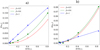 |
Fig. 5. Normalized errors, ε, defined by Eq. (48), in the velocity of charges as a function of the ratio between the integration time step Δt and ΔtCFL, accumulated after running the simulation until t = tF. Panel a: simulations of acoustic waves, and panel b: simulations of Alfvén waves. Blue triangles show results for β = 1 (defined in Eq. (21)); green circles are for β = 0.6, and red crosses are for β = 0.5. Solid lines show the results of quadratic polynomial fit ε = a(Δt/ΔtCFL)2 + b(Δt/ΔtCFL)+c, with coefficients given in Tables 4 and 5. |
Figure 5 shows that, as expected, the error between the analytical and the numerical solutions increases with the increase of the integration time step. However, this increase is different for different values of the parameter β. This parameter, defined in Eq. (21) determines the fraction of the implicit contribution to the numerical solution. For β = 1 the scheme is expected to be first-order accurate in time, and for β = 0.5 it is expected to be second-order accurate. In order to test if this is the case in our implementation, we performed a polynomial fit to the error function using the expression ε = a(Δt/ΔtCFL)2 + b(Δt/ΔtCFL)+c, with the constraint a ≥ 0. The values of the coefficients together with their standard deviation resulting from the fit are given in Table 4 for the acoustic waves and in Table 5 for the Alfvén waves. The results confirm that the polynomial fit to the numerical values is dominantly second order for β ≈ 0.5 and first order for β = 1. We also observe that while higher-order convergence of numerical schemes is generally desirable, the absolute value of the error for the β = 1 tests at a practical time step is of similar magnitude (acoustic waves) or smaller (Alfvén waves) than for the β ≈ 0.5 tests.
Values of the coefficients and their standard deviation of the polynomial fit of the error for the acoustic waves.
Values of the coefficients and their standard deviation of the polynomial fit of the error for the Alfvén waves.
It must be noted that the numerical solution here uses Δt up to the value dictated by the explicit single-fluid CFL condition. Therefore, we conclude that our implementation allows us to efficiently overcome the small time-step limitations implied by the stiff collisional terms in the two-fluid model.
5. Waves in a gravitationally stratified atmosphere
In this section we test the capabilities of the code to model waves in a strongly gravitationally stratified solar chromosphere. We assume a model atmosphere with all hydrodynamical parameters and purely horizontal magnetic field, Bx0, stratified in the vertical direction, z. The temperature is considered uniform (height-independent), and different for charges and neutrals. If we neglect viscosity, and consider only elastic collisions, adiabatic equation of energy, and ideal Ohm’s law, the linearized equations can be written as follows.
We separate the time dependence, assumed to be of the form exp(iωt) with constant ω, and combine the system into the equation of the vertical velocity for the charges: ucz(z, t) = ũcz(z)exp(iωt), obtaining a fourth-order ODE:
![$$ \begin{aligned}&\frac{\mathrm{d}^4 \tilde{u}_{\rm cz}}{\mathrm{d} z^4} a_{\rm c} a_{\rm n} + \frac{\mathrm{d}^3 \tilde{u}_{\rm cz}}{\mathrm{d} z^3} \left(a_{\rm n} b_{\rm c} + a_{\rm c} b_{\rm n} \right) \nonumber \\&\quad + \frac{\mathrm{d}^2 \tilde{ u_{\rm c}}_z}{\mathrm{d} z^2} \left[ b_{\rm c} b_{\rm n} + \omega ^2 \left(a_{\rm c} + a_{\rm n}\right) - i \alpha \omega (a_{\rm c} \rho _{\rm c0} + a_{\rm n} \rho _{\rm n0}) \right] \nonumber \\&\quad +\frac{\mathrm{d} \tilde{u}_{\rm cz}}{\mathrm{d} z} \omega \left[ \omega \left(b_{\rm c} + b_{\rm n}\right) - i \alpha \left(b_{\rm c} \rho _{\rm c0} + b_{\rm n} \rho _{\rm n0} \right) \right] \nonumber \\&\quad +u_{\rm cz} \omega ^3 \left[\omega - i \alpha \left(\rho _{\rm c0} + \rho _{\rm n0}\right) \right] =0 . \end{aligned} $$](/articles/aa/full_html/2019/07/aa34154-18/aa34154-18-eq78.gif)
where
The equilibrium variables for neutrals and for charges must fulfill the equations of state: Eq. (13) and the hydrostatic (HS) and magneto-hydrostatic (MHS) equilibrium conditions, respectively:
Since the temperature is assumed uniform, the pressure for neutrals has an exponential profile with a uniform scale height, and the sound speed of neutrals is constant. If we consider that the magnetic pressure has the same scale height as the pressure on the charges, after solving HS/MHS equations we obtain
with uniform scale heights:
The densities obtained from the ideal gas laws for neutrals and charges (Eq. (13)) also have an exponential profile. In these conditions, the quantities defined in Eq. (51), namely ac, n, bc, n = −ac, n/Hc, nn and α, are uniform; however, there are coefficients that explicitly contain density. We assumed that the scale of the height variation of the nonuniform coefficients in Eq. (50) is large compared to the oscillation wavelength, and therefore we can search for the solution in terms of plane waves, as

with Vc being the uniform real amplitude, and k the uniform complex wavenumber. The other variables are also in the form of plane waves (including the time dependence):
where Ṽn, R̃c, R̃n, P̃c,P̃n, and B̃ are uniform complex amplitudes. The following relations are obtained,
The dispersion relation is a fourth-order equation in ω:
In our particular case, the wavenumber k obtained from this space-dependent dispersion relation turns out to be almost uniform, and therefore we consider the plane wave solution to be a fair approximation.
5.1. Initial conditions
5.1.1. Equilibrium atmosphere
We choose the temperature for neutrals to be Tn0 = 6000 K. Further, for the number density of the neutrals and charges we use the values taken from the VALC (Vernazza et al. 1981) model at z0 ≈ 500 km: nc0(z0) = 5 × 10¹⁷ m−3, and nn0(z0) = 2.1 × 10²¹ m−3. In this test we take the temperature of the electrons into account; unlike the tests in the uniform atmosphere, they contribute to the pressure of charges and to collisions. We choose the value of Bx0(z0) = 10−4 T. In order to have the same scale height for neutrals and charges, we use the following temperature for the charges.
This gives the value of Tc0 ≈ 2422.47 K and Hn = Hc ≈ 1.8 × 10⁵ m. Subsequently, the pressures of charges and neutrals at z0, pc0(z0) and pn0(z0) are obtained from the ideal gas law (Eq. (13)). In these conditions, the wavenumber k obtained from the dispersion relation Eq. (56) is almost uniform, and has a value of k ≈ 1.383 × 10⁻⁴ + 2.767 × 10⁻⁶i m−1. Therefore, the wavelength is about four times shorter than the density scale height. The densities are calculated afterwards from the ideal gas laws for neutrals and charges (Eq. (13)), taking ρn0 = nnmH, ρc0 = nemH. We cover the domain Lz = 1.6 Mm with 32 000 grid points.
5.1.2. Perturbation
We choose the period of the wave to be P = 5 s, and calculate the frequency (ω = 2π/P) and the wavenumber (k) from the dispersion relation, Eq. (56). We choose the amplitude of the perturbation of the velocity of charges as a fraction of the background sound speed, Vc = 10−3c0, where

is the sound speed of the whole fluid, and its value is c0 ≈ 9.1 km s−1. We calculate the amplitudes of the other perturbations from the polarization relations, Eq. (55). The perturbation is generated by a driver at each time step in the ghosts points at the bottom of the atmosphere, which makes it the lower boundary condition. The perfectly matched layer (PML) is used as the upper boundary condition and is specially designed to absorb waves without reflections. It was first introduced for the first time for electromagnetic waves in the Maxwell equation by Berenger (1994), applied to Euler equations by Hu (1996), and to acoustic waves in a strongly stratified solar convection zone by Parchevsky & Kosovichev (2007). The description of the implementation of the PML in the Mancha code can be found in Felipe et al. (2010). In this test we have used the value of the scheme parameter β = 1.
5.2. Results
We run the code in two regimes. In the first case, we solved fully nonlinear equations for perturbations, and in the second case we evolved linearized equations where only the first-order terms were kept. The latter was done for comparison purposes, since the analytical solution assumes linear regime. We compare the numerical solutions at time t = 215.115 s with the analytical solution. At this time, simulations reached the stationary state, since the wave has reached the upper boundary and several periods of the wave have passed through the boundary. The results are shown in Figs. 6 and 7.
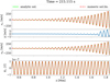 |
Fig. 6. Analytical solution (green solid line) and numerical linear solution (red dashed line) for the vertical velocity of charges (uzc) and neutrals (uzn), and for the perturbation in the x component of the magnetic field (B1x) for a snapshot taken in stationary state at t = 215.115 s. Below the panel showing the solutions for uzc, the difference between the numerical linear solution and the analytical solution for uzc is plotted. |
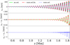 |
Fig. 7. First panel: analytical solution (green solid line) and numerical solutions: linear (red dashed line) and nonlinear (blue dotted line) for uzc for a snapshot taken in stationary state at t = 215.115 s. Second and third panels: decoupling (uzn − uzc) for the analytical and linear numerical solutions, and for the nonlinear numerical solutions, respectively. |
Figure 6 shows the analytical solution (green, solid line) superposed on the linear numerical solution (red, dashed line) for the vertical velocity of charges (uzc) in the first panel, the vertical velocity of neutrals (uzn) in the second panel, and for the perturbation in the x component of the magnetic field (Bx1) in the third panel. Below the panel of uzc we show the difference (Δ) between the linear numerical and the analytical solution of uzc. We observe that the numerical linear solution is in very good agreement with the analytical solution for the three quantities considered, and that the error is small (below 2%).
The first panel of Fig. 7 shows the nonlinear effects by superposing the nonlinear numerical solution (blue, dotted line) of uzc along with the analytical solution (green solid line) and the linear numerical solution (red dashed line), for the same snapshot taken at t = 215.115 s. In the second and third panels we show the decoupling in the vertical velocity (unz − ucz) for the analytical and linear solutions superposed, and the nonlinear solution, respectively.
We observe that the wave profile steepens at the end of the domain when the amplitude becomes large and nonlinear effects are visible in the case of the nonlinear solution. As a consequence, the amplitude of the wave is smaller than in the linear case (see e.g., Landau & Lifshitz 1987). Wave amplitude grows with height in a gravitationally stratified atmosphere because of the density decrease. In the case considered here, the damping is not large enough to overcome this growth,and therefore the wave evolves into a shock. The amplitude growth is nevertheless below the growth in the MHD limit.
We also observe that the decoupling predicted analytically from the relation between Ṽn and Vc in Eq. (55) agrees with the decoupling obtained from the linear numerical simulation. In order to intuitively understand the reason for the linear decoupling, we show in Fig. 8 the relevant frequencies corresponding to this problem. Even though the collisional parameter α is uniform because of the uniform background temperature of neutrals and charges, and has the value ≈4.1 × 10¹¹ m3 kg−1 s−1, the collision frequency also depends on density (Eq. (5)), and has an exponential profile. While for the charges the collision frequency νcn is larger than both the ion-cyclotron frequency (ωci) and the wave frequency (which determine the hydrodynamical timescale), for the neutrals the neutral-charges collision frequency goes from being greater than the wave frequency to being less than the wave frequency at a point located at z ≈ 1.4 Mm in the atmosphere. This is the point after which we observe the decoupling for the linear numerical solution and the analytical solution. The code efficiently captures the transition from a coupled to a partially decoupled regime. In the nonlinear case, the hydrodynamical timescale is smaller than in the linear case. The shock front width, which determines the hydrodynamical space scale in the nonlinear case, is smaller than the wavelength. The nonlinear decoupling appears spatially at the shock front, and is almost five times larger than the linear decoupling.
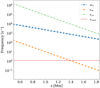 |
Fig. 8. Relevant frequencies: ion-cyclotron frequency: ωci (blue dashed line marked with diamonds), wave frequency: νwave = 2π/Pwave (red solid line), neutral-charge collision frequency: νnc (orange dotted line marked with circles), and charge-neutral collision frequency: νcn (green dotted line marked with “X”). |
6. Discussion and conclusions
Strong vertical and horizontal stratification in solar atmospheric plasma parameters makes theoretical modeling of the solar chromosphere particularly complicated, where it is expected that the collisional timescales between charged and neutral plasma components may become similar or longer than MHD timescales, leading to a breakdown of the single-fluid MHD approximation. In such conditions, neutrals start to decouple from charges, behaving as two independent fluids. This work describes the results of our numerical effort to extend the existing single-fluid nonlinear MHD code MANCHA3D for modeling of solar plasma dynamics under the two-fluid approximation. To this end, we implemented a semi-implicit numerical scheme following the approach by Toth et al. (2012). Such development is a necessary and logical step towards creation of a 3D modeling tool for simulations of multi-component plasma processes in the solar chromosphere.
As discussed in the Introduction, the collisional terms in the upper layers of the solar atmosphere have values similar to the rest of the forces in the momentum equation. In the lower layers (photosphere) their values significantly dominate over the rest of the terms. However, coupling between these layers plays an important role in the energy and momentum transfer from the solar interior to the corona, and therefore it is necessary to create numerical tools that would be able to treat both extreme situations in a single simulation domain. Classical explicit schemes would be limited by the explicit time step dictated by the CFL condition due to collisional terms, making it very small and significantly slowing the numerical code. A suitable alternative suggested by Toth et al. (2012) is a semi-implicit implementation. This implementation allowed us to keep the advantages of an explicit code (efficient parallelization and lower memory requirements), but at the same time to overcome the restrictions imposed by small collisional times. We based our implementation on the already existing numerical code, MANCHA3D, and were therefore able to keep all its already implemented functionalities such as hyper-diffusivities, noise-filtering modules, PML boundary condition, and parallelization.
Several features of our numerical code, such as shock resolving, have previously been thoroughly tested (Khomenko & Collados 2006, 2012; Felipe et al. 2010; González-Morales et al. 2018). The particular effort in this work was to verify the performance of the semi-implicit fluid-coupling algorithm. To this end we compared the numerical solution with the known analytical solutions for propagation of acoustic and Alfvén waves in a homogeneous plasma with a different degree of collisional coupling.
Our analytical results are similar to those obtained by Zaqarashvili et al. (2011b) and Soler et al. (2013a). When the temperatures of charges and neutrals are initially different, if the ratio α/k is small, the acoustic waves in each of the fluids propagate nearly independently of each other with their respective sound speeds. The Alfvén waves propagate with the Alfvén speed of the charged fluid if the collisional coupling is weak. In the opposite limit, when the ratio α/k is large, the two fluids become coupled. The acoustic waves propagate with the sound speed of the whole fluid, and the Alfvén waves propagate with the Alfvén speed calculated using the total atom mass density. In this case, the velocities of neutrals and charges are of equal amplitude and are in phase. At these two extremes, when the quantity αρtot/(kctot) is either low or high, the waves have little damping relative to wavenumber, but when the collisional frequency is of the order of the wave frequency the damping relative to wavenumber is maximum.
Our numerical solution reproduces the analytical solution for the full range of the values of the wavenumber k. The temporal convergence tests have shown that, as expected, the newly implemented scheme is first-order accurate when the scheme parameter β = 1, and is second-order accurate when β ≈ 0.5. However, we note that even if the scheme converges linearly with Δt for the scheme parameter β = 1, the overall behavior of the scheme is more stable, and the errors are in fact smaller.
Our current study must be viewed in the context of other similar developments by other groups of authors. There have been several approaches proposed to overcome the limitations introduced by large collisional terms.
Hillier et al. (2016) noticed that since collisional terms introduce a very different timescale, the solution can be obtained semi-analytically. In their approach, the equations with only collisional terms are solved analytically and then the rest of the terms are evolved numerically using an explicit scheme. When the hydrodynamical and the collisional timescales are similar, only the explicit scheme is applied. Such an approach has a drawback since the entire numerical domain has to be placed in one regime or the other, and therefore it may cause problems when strong stratification in the atmosphere is present. In our case, there is no need to have a criterion to distinguish between these regimes; the scheme handles both of them well and in the same way. Convergence tests were carried out for the coupled regime, and the errors were shown to be larger. The neutrals and charges are more coupled at larger values of the ratio α/k. We have seen from the convergence test that the scheme behaves better in the strongly coupled regime for the values of the scheme parameter β closer to 1 than to 0.5, and this is the reason for choosing this value for the last test. The last test, the simulation in the gravitationally stratified atmosphere, deals with the situation where the waves pass from a collisionally coupled regime to a decoupled regime, and the numerical results are satisfactory.
Alternatively, Maneva et al. (2017) used a fully implicit scheme which has no restriction for the time-step and is generally more stable. It must be noted that despite the advantage of the stability, implicit schemes are more computationally expensive because generally the matrix inversions needed in the implicit part are implemented by iterations, increasing the computational time. However, if one only deals with the collisional terms such as Sn, Rn and Mn in Eqs. (2), (6), and (10), there is an important advantage since these terms are linear with respect to the main set of variables and do not contain derivatives. Therefore, the matrix inversion can be done fully analytically, improving the precision and the computational capabilities of the implicit code. Such an analytical approach is not possible when dealing with physical effects such as thermal conduction or viscosity. In general, semi-implicit implementations such as the one presented here are less computationally expensive, but are also less accurate than fully implicit ones.
Similarly to our method, Smith & Sakai (2008) implemented the collisional terms following a semi-implicit approach. Smith & Sakai (2008) used a two-fluid code, where they considered the plasma composed by ions and neutrals, and they implemented most of the collisional terms in a scheme similar to that of Toth et al. (2012) with a β parameter equal to 1. These authors considered ionization/recombination terms in continuity and momentum equations, elastic collisions in momentum equations, and the work done by the collisional terms in the energy equations. However, unlike our implementation, they did not consider the inelastic collision terms, the thermal exchange, or the frictional heating in the energy equations.
Yet another widely used code for multi-fluid simulations is the HiFi code by Lukin et al. (2016), which uses an implicit temporal discretization and spectral element spatial decomposition. This code has been extensively used for simulations of reconnection in partially ionized plasma (Leake et al. 2012, 2013; Ni et al. 2018) and has similar advantages and drawbacks to the implicit implementation discussed above.
All in all, the above implementations have their advantages and disadvantages. In our case, we have chosen a semi-implicit approach because the collisional terms that need to be implemented implicitly, are linear in the variables that evolve in time, and the implicit solution can be obtained analytically. The tests we carried out in order to verify the code showed satisfactory results.
While the present paper only presents calculations in cases where analytical solutions exist and can be compared to the numerical solution, our forthcoming results described in Paper II (Popescu Braileanu et al. 2019) demonstrate that the newly implemented algorithm is able to efficiently deal with chromospheric gravitational stratification and can be used for modeling of propagation of chromospheric shock waves under the two-fluid framework.
Acknowledgments
This work was supported by the Spanish Ministry of Science through the project AYA2014-55078-P and the US National Science Foundation. It contributes to the deliverable identified in FP7 European Research Council grant agreement ERC-2017-CoG771310-PI2FA for the project “Partial Ionization: Two-fluid Approach”. The author(s) wish to acknowledge the contribution of Teide High-Performance Computing facilities to the results of this research. TeideHPC facilities are provided by the Instituto Tecnológico y de Energías Renovables (ITER, SA), http://teidehpc.iter.es
References
- Alvarez Laguna, A., Lani, A., Poedts, S., Mansour, N. N., & Kosovichev, A. G. 2014, AGU Fall Meeting Abstracts [Google Scholar]
- Anan, T., Ichimoto, K., & Hillier, A. 2017, A&A, 601, A103 [NASA ADS] [CrossRef] [EDP Sciences] [Google Scholar]
- Athay, R. G., & House, L. L. 1962, ApJ, 135, 500 [NASA ADS] [CrossRef] [Google Scholar]
- Ballester, J. L., Alexeev, I., Collados, M., et al. 2018, Space Sci. Rev., 214, 58 [NASA ADS] [CrossRef] [Google Scholar]
- Berenger, J. P. 1994, J. Comp. Phys., 114, 185 [CrossRef] [Google Scholar]
- Braginskii, S. I. 1965, Rev. Plasma Phys., 1, 205 [Google Scholar]
- de la Cruz Rodríguez, J., & Socas-Navarro, H. 2011, A&A, 527, L8 [NASA ADS] [CrossRef] [EDP Sciences] [Google Scholar]
- Felipe, T., Khomenko, E., & Collados, M. 2010, ApJ, 719, 357 [Google Scholar]
- Gilbert, H. R., Hansteen, V. H., & Holzer, T. E. 2002, ApJ, 577, 464 [NASA ADS] [CrossRef] [Google Scholar]
- Gilbert, H., Kilper, G., & Alexander, D. 2007, ApJ, 671, 978 [NASA ADS] [CrossRef] [Google Scholar]
- González-Morales, P. A., Khomenko, E., Downes, T. P., & de Vicente, A. 2018, A&A, 615, A67 [NASA ADS] [CrossRef] [EDP Sciences] [Google Scholar]
- Hillier, A., Takasao, S., & Nakamura, N. 2016, A&A, 591, A112 [NASA ADS] [CrossRef] [EDP Sciences] [Google Scholar]
- Hu, F. Q. 1996, J. Comp. Phys., 129, 201 [Google Scholar]
- Khomenko, E., & Collados, M. 2006, ApJ, 653, 739 [Google Scholar]
- Khomenko, E., & Collados, M. 2012, ApJ, 747, 87 [NASA ADS] [CrossRef] [Google Scholar]
- Khomenko, E., Collados, M., Díaz, A., & Vitas, N. 2014, Phys. Plasmas, 21, 092901 [NASA ADS] [CrossRef] [Google Scholar]
- Khomenko, E., Collados, M., Shchukina, N., & Díaz, A. 2015, A&A, 584, A66 [NASA ADS] [CrossRef] [EDP Sciences] [Google Scholar]
- Khomenko, E., Collados, M., & Díaz, A. J. 2016, ApJ, 823, 132 [NASA ADS] [CrossRef] [Google Scholar]
- Landau, L. D., & Lifshitz, E. M. 1987, in Fluid Mechanics: Course of Theoretical Physics, 2nd edn., eds. L. D. Landau, & E. M. Lifshitz (Oxford: Butterworth-Heinemann), 6 [Google Scholar]
- Leake, J. E., Lukin, V. S., Linton, M. G., & Meier, E. T. 2012, ApJ, 760, 109 [NASA ADS] [CrossRef] [Google Scholar]
- Leake, J. E., Lukin, V. S., & Linton, M. G. 2013, Phys. Plasmas, 20, 061202 [NASA ADS] [CrossRef] [Google Scholar]
- Leenaarts, J. 2010, Mem. Soc. Astron. It., 81, 576 [NASA ADS] [Google Scholar]
- Lukin, V. S., Glasser, A. H., Lowrie, W., & Meier, E. T. 2016, ArXiv e-prints [arXiv:1608.06030] [Google Scholar]
- Maneva, Y. G., Alvarez Laguna, A., Lani, A., & Poedts, S. 2017, ApJ, 836, 197 [NASA ADS] [CrossRef] [Google Scholar]
- Martínez-Sykora, J., De Pontieu, B., Carlsson, M., & Hansteen, V. 2016, ApJ, 831, L1 [NASA ADS] [CrossRef] [Google Scholar]
- Martínez-Gomez, D., Soler, R., & Terradas, J. 2017, ApJ, 837, 80 [NASA ADS] [CrossRef] [Google Scholar]
- Meier, E. T., & Shumlak, U. 2012, Phys. Plasmas, 19, 072508 [NASA ADS] [CrossRef] [Google Scholar]
- Ni, L., Lukin, V. S., Murphy, N. A., & Lin, J. 2018, ApJ, 852, 95 [NASA ADS] [CrossRef] [Google Scholar]
- Nye, A. H., & Thomas, J. H. 1976, ApJ, 204, 573 [NASA ADS] [CrossRef] [Google Scholar]
- Parchevsky, K. V., & Kosovichev, A. G. 2007, ApJ, 666, L53 [NASA ADS] [CrossRef] [Google Scholar]
- Popescu Braileanu, B., Lukin, V. S., Khomenko, E., & de Vicente, A. 2019, ArXiv e-prints [arXiv: 1905.03559] [Google Scholar]
- Rempel, M., Schüssler, M., & Knölker, M. 2009, ApJ, 691, 640 [NASA ADS] [CrossRef] [Google Scholar]
- Smirnov, B. M. 2003, XII, I, 443 [Google Scholar]
- Smith, P. D., & Sakai, J. I. 2008, A&A, 486, 569 [NASA ADS] [CrossRef] [EDP Sciences] [Google Scholar]
- Soler, R., Carbonell, M., Ballester, J. L., & Terradas, J. 2013a, ApJ, 767, 171 [NASA ADS] [CrossRef] [Google Scholar]
- Soler, R., Diaz, A. J., Ballester, J. L., & Goossens, M. 2013b, A&A, 551, A86 [NASA ADS] [CrossRef] [EDP Sciences] [Google Scholar]
- Toth, G., van der Holst, B., Sokolov, I. V., et al. 2012, J. Comput. Phys., 231, 870 [Google Scholar]
- Vernazza, J. E., Avrett, E. H., & Loeser, R. 1981, ApJS, 45, 635 [NASA ADS] [CrossRef] [Google Scholar]
- Vögler, A., Shelyag, S., Schüssler, M., et al. 2005, A&A, 429, 335 [NASA ADS] [CrossRef] [EDP Sciences] [Google Scholar]
- Voronov, G. 1997, At. Data Nucl. Data Tables, 65, 1 [Google Scholar]
- Zaqarashvili, T. V., Khodachenko, M. L., & Rucker, H. O. 2011a, A&A, 534, A93 [NASA ADS] [CrossRef] [EDP Sciences] [Google Scholar]
- Zaqarashvili, T. V., Khodachenko, M. L., & Rucker, H. O. 2011b, A&A, 529, A82 [NASA ADS] [CrossRef] [EDP Sciences] [Google Scholar]
- Zaqarashvili, T. V., Khodachenko, M. L., & Soler, R. 2013, A&A, 549, A113 [NASA ADS] [CrossRef] [EDP Sciences] [Google Scholar]
Appendix A: Expressions of terms
A.1. Collisions
Expressions for Γion and Γrec as functions of ne and Te are given in Voronov (1997) and Smirnov (2003):
where ϕion = 13.6 eV,  is electron temperature in eV, A = 2.91 × 10⁻¹⁴, K = 0.39, and X = 0.232.
The elastic collisional frequency between particles of species α and particles of species β is expressed as (see e.g., Braginskii 1965)
We highlight the fact that ναβ ≠ νβα, but ραναβ = ρβνβα. In the expression for collisional frequency, Tαβ = (Tα + Tβ)/2 is the average temperature, and mαβ = mαmβ/(mα + mβ) is the reduced mass of particles α and β.
The elastic collisional parameter α defined in Eq. (4) has the form
The charge-exchange (elastic) collisional parameter between particles of species α (ions) and particles of species β (neutrals) is approximately expressed as (see, e.g. Meier & Shumlak 2012):
with
where vTα, and vrelαβ are the thermal velocity of particles of species α, and the module of the relative velocity between particles of species α and particles of species β is respectively
If charge-exchange reactions are taken into account, the effective elastic collisional parameter is
A.2. Viscosities and thermal conductivities
(derived by Braginskii 1965):

Replacing for the collisional frequency, the above equations can be written as
This leads the viscosity and thermal conduction coefficient to depend only on the temperature. For the viscosity and thermal conductivity of the charges, only the ions are taken into account.
The collisional cross sections used were: Σnn = 2.1 × 10⁻¹⁸ m2,  , where e is the elementary charge, and ϵ0 the permitivity of free space, Σin = 1.16 × 10⁻¹⁸ m2, and Σen = 10−19 m2.
mn = mH is the mass of the hydrogen atom.
Appendix B: Analytical expressions of the Jacobian
The analytical expressions of the Jacobian where we use the superscripts D, M, and E for the continuity, momentum, and energy equations, respectively, are
B.1. Continuity equations
B.2. Momentum equations
B.3. Energy equations
where A = 2 when the temperature of the electrons is taken into account, and A = 1 when temperature of the electrons is not taken into account.

All Tables
Values of the background atmosphere parameters used in the tests of the wave propagation in the uniform medium for neutrals (left) and charges (right).
Values of the coefficients and their standard deviation of the polynomial fit of the error for the acoustic waves.
Values of the coefficients and their standard deviation of the polynomial fit of the error for the Alfvén waves.
All Figures
|
Fig. 1. Solutions of the dispersion relation, Eq. (31), for the acoustic wave case. Left and right panels present the real and imaginary parts of the dimensionless wave frequency ω, respectively, as functions of the dimensionless wavenumber k. The axes are scaled in nondimensional units E and F, defined in Eq. (32) for better visualization. Four solutions are marked with different colors and line styles: solid red for solution 1, orange dashed for solution 2, blue dot-dashed for solution 3, and green dotted for solution 4. We note that solutions 1 and 4 have the same imaginary parts and are superposed in the right-hand panel. Solutions 2 and 3 have the same real part equal to zero for large α/k and are also superimposed on top of one another. The values of k for which we compare the analytical and numerical solution using the values of ω, corresponding to solution 4 (green dots), are marked in the panels: orange circle (k = 618 m−1), pink triangle (k = 6.18 m−1), cyan diamond (k = 2.06 m−1), and black “X” (k = 6.18 × 10⁻⁶ m−1). |
| In the text | |
|
Fig. 2. Solutions of the dispersion relation, Eq. (39), for the Alfvén wave case. Left and right panels present the real and imaginary parts of the wave frequency ω, respectively, as a function of the wavenumber k. The axes are scaled in the nondimensional units: C and D, defined in Eq. (40) for better visualization. Three solutions are marked with different colors and line styles: red solid for solution 1, orange dashed for solution 2, and green dotted for solution 3. The values of k for which we compare the analytical and numerical solutions using the values of ω, corresponding to solution 3 (green dots), are marked in the panels: pink triangle (k = 61.8 m−1), green triangle (k = 6.18 m−1), orange star (k = 6.18 × 10⁻² m−1), and black triangle (k = 6.18 × 10⁻⁶ m−1). |
| In the text | |
|
Fig. 3. Simulations of acoustic wave propagation in a homogeneous plasma. Numerically (red dashed line) and analytically (green solid line) calculated time evolution of the velocity of neutrals and charges as a function of time. Below the panels showing the velocity of neutrals, the difference (Δ) between the numerical solution and the analytical solution for unz is given. Time is measured in units of the wave period, 2π/ωR. Panels from left to right and from top to bottom: simulations for different values of the wavenumber k, as indicated in the legend of Fig. 1. |
| In the text | |
|
Fig. 4. Simulations of Alfvén wave propagation in a homogeneous plasma. Here we show the numerically (red dashed line) and analytically (green solid line) calculated time evolution of the velocity of neutrals and charges, and the magnetic field perturbation, as a function of time. Below the panels showing the velocity of charges, the difference (Δ) between the numerical solution and the analytical solution for ucx is plotted. Time is measured in units of the wave period, 2π/ωR. Panels from left to right and from top to bottom: simulations for different values of the wavenumber k, as indicated in the legend of Fig. 2. |
| In the text | |
|
Fig. 5. Normalized errors, ε, defined by Eq. (48), in the velocity of charges as a function of the ratio between the integration time step Δt and ΔtCFL, accumulated after running the simulation until t = tF. Panel a: simulations of acoustic waves, and panel b: simulations of Alfvén waves. Blue triangles show results for β = 1 (defined in Eq. (21)); green circles are for β = 0.6, and red crosses are for β = 0.5. Solid lines show the results of quadratic polynomial fit ε = a(Δt/ΔtCFL)2 + b(Δt/ΔtCFL)+c, with coefficients given in Tables 4 and 5. |
| In the text | |
|
Fig. 6. Analytical solution (green solid line) and numerical linear solution (red dashed line) for the vertical velocity of charges (uzc) and neutrals (uzn), and for the perturbation in the x component of the magnetic field (B1x) for a snapshot taken in stationary state at t = 215.115 s. Below the panel showing the solutions for uzc, the difference between the numerical linear solution and the analytical solution for uzc is plotted. |
| In the text | |
|
Fig. 7. First panel: analytical solution (green solid line) and numerical solutions: linear (red dashed line) and nonlinear (blue dotted line) for uzc for a snapshot taken in stationary state at t = 215.115 s. Second and third panels: decoupling (uzn − uzc) for the analytical and linear numerical solutions, and for the nonlinear numerical solutions, respectively. |
| In the text | |
|
Fig. 8. Relevant frequencies: ion-cyclotron frequency: ωci (blue dashed line marked with diamonds), wave frequency: νwave = 2π/Pwave (red solid line), neutral-charge collision frequency: νnc (orange dotted line marked with circles), and charge-neutral collision frequency: νcn (green dotted line marked with “X”). |
| In the text | |
Current usage metrics show cumulative count of Article Views (full-text article views including HTML views, PDF and ePub downloads, according to the available data) and Abstracts Views on Vision4Press platform.
Data correspond to usage on the plateform after 2015. The current usage metrics is available 48-96 hours after online publication and is updated daily on week days.
Initial download of the metrics may take a while.