| Issue |
A&A
Volume 612, April 2018
|
|
|---|---|---|
| Article Number | A20 | |
| Number of page(s) | 11 | |
| Section | Stellar structure and evolution | |
| DOI | https://doi.org/10.1051/0004-6361/201731969 | |
| Published online | 13 April 2018 | |
Global hot-star wind models for stars from Magellanic Clouds
1
Ústav teoretické fyziky a astrofyziky PřF MU,
611 37
Brno, Czech Republic
e-mail: This email address is being protected from spambots. You need JavaScript enabled to view it.
2
Astronomický ústav, Akademie věd České republiky,
251 65
Ondřejov, Czech Republic
Received:
19
September
2017
Accepted:
5
December
2017
Abstract
We provide mass-loss rate predictions for O stars from Large and Small Magellanic Clouds. We calculate global (unified, hydrodynamic) model atmospheres of main sequence, giant, and supergiant stars for chemical composition corresponding to Magellanic Clouds. The models solve radiative transfer equation in comoving frame, kinetic equilibrium equations (also known as NLTE equations), and hydrodynamical equations from (quasi-)hydrostatic atmosphere to expanding stellar wind. The models allow us to predict wind density, velocity, and temperature (consequently also the terminal wind velocity and the mass-loss rate) just from basic global stellar parameters. As a result of their lower metallicity, the line radiative driving is weaker leading to lower wind mass-loss rates with respect to the Galactic stars. We provide a formula that fits the mass-loss rate predicted by our models as a function of stellar luminosity and metallicity. On average, the mass-loss rate scales with metallicity as Ṁ ~ Z0.59. The predicted mass-loss rates are lower than mass-loss rates derived from Hα diagnostics and can be reconciled with observational results assuming clumping factor Cc = 9. On the other hand, the predicted mass-loss rates either agree or are slightly higher than the mass-loss rates derived from ultraviolet wind line profiles. The calculated P v ionization fractions also agree with values derived from observations for LMC stars with Teff ≤ 40 000 K. Taken together, our theoretical predictions provide reasonable models with consistent mass-loss rate determination, which can be used for quantitative study of stars from Magellanic Clouds.
Key words: stars: winds, outflows / stars: mass-loss / stars: early-type / Magellanic Clouds / hydrodynamics / radiative transfer
© ESO 2018
1 Introduction
The radiative force influences various types of astrophysical objects on different spatial scales. Because the radiative force acts selectively on individual species, it depends on their abundances, and consequently also on metallicity. The metallicity dependence of radiatively driven hot-star winds leads to the absence of line-driven outflows in metal-free Pop III stars (Krtička & Kubát 2006), while Galactic stars lose a significant part of their mass due to the winds (e.g., Keszthelyi et al. 2017).
Besides metallicity, hot-star wind mass-loss rates depend also on other basic stellar parameters (luminosity, mass, and radius). While dependence of hot-star wind on most of the stellar parameters can be observationally studied using a local stellar sample (e.g., Puls et al. 2006), similar study of metallicity dependence is more complicated. Besides ultraviolet (UV) satellites, observational study of mass loss at a fraction of the solar metallicity in the Magellanic Clouds requires large telescopes. It was possible to extend the range of studied metallicities using spectroscopic observations of stars residing in galaxies of the Local Group (Tramper et al. 2011; Herrero et al. 2012). However, hot stars with metallicity below about one tenth of the solar metallicity are still observationally unattainable for a detailed wind study.
The most complete picture of the dependence of wind properties on the metallicity can be therefore obtained from theoretical models. Such models are able to predict the dependence of basic wind properties on metallicity. The most important wind parameter is the mass-loss rate Ṁ, that is the amount of mass lost by the star per unit of time. Vink et al. (2001) predicted that for a broad range of metallicities Z (given by the mass fraction of heavier elements) the mass-loss rate varies as Ṁ ~ Z0.69 in O and early B stars. A more complex dependence of the mass-loss rate on metallicity was found by Gräfener & Hamann (2008) for late-type WN stars. Petrov et al. (2016) calculated metallicity-dependent wind mass-loss rates from the balance between the radiative energy deposited in the wind and the energy required to lift up the wind material. The latter calculations based on the CMFGEN code predicted that the metallicity dependence of the mass-loss rate in luminous B stars is a complicated function of stellar effective temperature and is the strongest around Teff = 17 500–20 000 K.
Study of stellar winds at very low metallicities is important for understanding stellar evolution and stellar feedback in the early Universe and in dwarf galaxies from the Local Group. The gravitational-wave source GW150914 is also expected to originate from low-metallicity environment (Abbott et al. 2016). Because observations of stars in such low-metallicity environments are not always possible, the numerical models may provide missing information about the wind physics. To reach this goal, the current models have to be tested against observations for as broad a range of metallicities as possible.
However, testing of wind models at low metallicities is complicated by the mismatch between individual mass-loss rate determinations. Even at Galactic metallicity the estimates based on the X-ray spectroscopy (Cohen et al. 2014; Rauw et al. 2015), combined optical and UV analysis (Bouret et al. 2012; Šurlan et al. 2013), and near-infrared line spectroscopy (Najarro et al. 2011) seem to point to lower mass-loss rates than predicted by Vink et al. (2001). On the other hand, the results based purely on the Hα emission lines (Mokiem et al. 2007b) can be reconciled with theoretical predictions of Vink et al. (2001). Moreover, a multiwavelength analysis of Shenar et al. (2015) shows good agreement with theoretical models. Consequently, the existence of the discrepancy between empirical and theoretical mass-loss rate determinations is not unanimously accepted. The discrepancy may be evennonmonotonic, because massive stars at the top of the main sequence show enhanced mass-loss rates with respect to theoretical models (Bestenlehner et al. 2014).
Part of these discrepancies may be connected with the influence of inhomogeneities on the observational mass-loss rate diagnostics (Sundqvist et al. 2010, 2011; Šurlan et al. 2012, 2013) and on theoretical predictions (Muijres et al. 2011; Sundqvist et al. 2014). On the other hand, wind blocking in global (unified) wind models leads to reduction of predicted mass-loss rates in agreement with some observational estimates (Krtička & Kubát 2017). These mass-loss rates taken from global wind models are typically lower than Vink et al. (2001) and Pauldrach et al. (2012) mass-loss rates by a factor of 2–5, however they are consistent with predictions based on CMFGEN (Bouret et al. 2012; Puebla et al. 2016; Petrov et al. 2016)and PoWR codes (Gräfener 2003; Sander et al. 2017). Here we apply our global wind models (Krtička & Kubát 2017) to stars from Magellanic Clouds.
2 Description of global wind models
The wind models used here were calculated using the METUJE code (Krtička & Kubát 2010, 2017), which provides global (unified) models of the stellar photosphere and wind. The code solves the radiative transfer equation, the kinetic (statistical) equilibrium equations, and hydrodynamic equations (equations of continuity, momentum, and energy) both in the photosphereand in the wind. The code assumes that the flow is stationary (time-independent) and spherically symmetric.
The radiative transfer equation is solved in the comoving frame (CMF) following the method proposed by Mihalas et al. (1975). We include line and continuum transitions relevant in atmospheres of hot stars in the radiative transfer equation. The inner boundary condition for the radiative transfer equation is derived from the diffusion approximation, and we assume no infalling radiation at the outer boundary.
The ionization and excitation state of considered elements was calculated from the kinetic equilibrium equations (also called NLTE equations). These equations account for the radiative and collisional excitation, deexcitation, ionization, and recombination. Part of the models of ions was adopted from the TLUSTY model stellar atmosphere input data (Lanz & Hubeny 2003, 2007). To prepare the remaining ionic models listed in Krtička & Kubát (2009) and not included in TLUSTY input data we use the same strategy as in TLUSTY, that is, the data are based on the Opacity and Iron Project calculations (Seaton et al. 1992; Hummer et al. 1993) and corrected by the observational data available in the NIST database (Kramida et al. 2015). For phosphorus the ionic model was prepared using data described by Pauldrach et al. (2001). The low-lying levels of ions are included explicitly in the calculations, while the higher levels are merged into superlevels (see Lanz & Hubeny 2003, 2007, for details). The bound-free radiative rates are consistently calculated from the CMF mean intensity, while for the bound–bound rates we still use the Sobolev approximation.
Three different methods are needed to solve the energy equation. We use a differential form of the transfer equation deep in the photosphere, while the integral form of this equation is advantageous in the upper layers of the photosphere (Kubát 1996). The electron thermal balance method (Kubát et al. 1999) is applied in the wind. The individual terms in the energy equation are taken from the CMF radiative field. The hydrodynamical equations, that is, the continuity equation, equation of motion, and the energy equation, are solved iteratively to obtain the wind density, velocity, and temperature structure. The iterations of hydrodynamical equations are performed using the Newton–Raphson method (see Fig. 1 for convergence properties). The derivatives of the CMF radiative force with respect to the flow variables within the Newton–Raphson iteration step are approximated from the line force in the Sobolev approximation corrected by the CMF line force (Krtička & Kubát 2010). We use the “shooting method” to derive an estimate of the mass-loss rate. We calculate a series of wind models with variable base velocity and search for the base velocity which provides a smooth transonic solution with maximum mass-loss rate (Krtička & Kubát 2017). The radiative force due to line and continuum transitions is calculated in the CMF. The line data for the calculation of the line force were taken from the VALD database (Piskunov et al. 1995; Kupka et al. 1999) with some updates using the NIST data (Kramida et al. 2015).
We utilize the TLUSTY model stellar atmospheres (Lanz & Hubeny 2003, 2007) to derive the initial guess of the solution in the photosphere. The TLUSTY models are calculated for the same effective temperature, surface gravity, and chemical composition as the wind models.
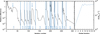 |
Fig. 1 Convergence of the hydrodynamical structure of the LMC 400-3 model. Left plot: maximum relative difference between hydrodynamical variables in subsequent iteration steps as a function of total number of hydrodynamical iterations. We note that kinetic equilibrium equations are iterated for each step of hydrodynamical iterations. Blue vertical strips denote a new step of a global iteration (numbered in the bottom of the plot) when the inner boundary velocity (and the mass-loss rate) is changed. Labels a–d in the bottom of the plot indicate (see also Krtička & Kubát 2017, Sect. 2): Panel a:calculation of the initial model for subcritical velocities. In the first few steps the CMF radiative transfer is not solved. Afterwards, the CMF calculations are switched on (indicated by a blue arrow). Panel b: iteration of wind model with mass-loss rate lower than or equal to the final one. Each model denoted as b has a higher mass-loss rate than the previous one. Panel c: iteration of wind model with mass-loss rate lower than the final one and inclusion of model for supercritical velocities. Here the blue arrow denotes inclusion of model for supercritical velocities. Panel d: iteration of wind model with mass-loss rate higher than the final one. After this step the model mass-loss rate decreases. The plot shows that the convergence of hydrodynamical structure in each step is stable and relatively fast. Right plot: mass-loss rate in individual global iteration steps (numbers on horizontal axis are the same as in blue labels in the left plot). The models converge to a final mass-loss rate given in Table 1. |
Stellar parameters of the model grid with derived values of the terminal velocity v∞ and mass-lossrate Ṁ.
3 Calculated global wind models
We calculated a grid of global wind models for metallicities corresponding to Magellanic Cloud O stars in the effective temperature range 30 000–45 000 K. Stellar masses and radii given in Table 1 were calculated using relations of Martins et al. (2005) for main sequence stars, giants, and supergiants. Although these relations were derived for Galactic stars, they fairly describe also the parameters of stars from Magellanic Clouds (cf., Massey et al. 2005; Mokiem et al. 2007a). We assumed solar chemical composition (Asplund et al. 2009) scaled for elements heavier than helium by a factor of 0.5 and 0.2 corresponding to typical chemical composition of stars in Large and Small Magellanic Clouds (e.g., Hill et al. 1995; Venn 1999; Rolleston et al. 2002; Bouret et al. 2003), respectively.
The photospheric structure of METUJE global models in Figs. A.1 and A.3 nicely agrees with results of the hydrostatic planparallel TLUSTY code. The agreement is even slightly better than for Galactic stars, which is likely caused by lower iron abundance, consequently by lower influence of iron lines on temperature. The METUJE and TLUSTY emergent fluxes in Figs. A.2 and A.4 also reasonably agree, with the exception of the frequency region above roughly 7 × 10¹⁵ s−1 where the flux is blocked by the wind. This blocking is weaker for winds with lower mass-loss rates. Larger differences appear in He ii Lymancontinuum (see Figs. A.2 and A.4), because the continuum originates in the wind. The differences in He ii Lyman continuum are lower for the hottest stars, where helium is nearly completely ionized.
The derived mass-loss rates are given in Table 1. Together with mass-loss rates calculated for Galactic O stars (Krtička & Kubát 2017), their metallicity dependence can be fitted using the formula
![Mathematical equation: \begin{eqnarray*} \log{\left({\frac{\dot M}{1\, {\ensuremath{{\ensuremath{{M}_{\odot}}}\,\text{yr}^{-1}}} }}\right)}&=& - 5.70+ 0.50 \log{\left({\frac{Z}{Z_{\odot}}}\right)} \\* && + {\left[{1.61- 0.12 \log{\left({\frac{Z}{Z_{\odot}}}\right)}}\right]} \log{\left({\frac{L}{10^6\,L_{\odot}}}\right)}.\end{eqnarray*}](/articles/aa/full_html/2018/04/aa31969-17/aa31969-17-eq1.png)
The fit provides relatively accurate approximation of our results with a typical error of about 10–30%. Because the Teff range of calculated Galactic O star wind models is narrower, the formula is valid for Teff = 30 000–42 500 K for Z∕Z⊙ = 0.2–1, while at Magellanic Cloud metallicities can be used up to Teff = 45 000 K. Equation (1) shows that with decreasing metallicity not only does the mass-loss rate decrease due to weaker line force, but also the luminosity dependence becomes steeper. The steeper luminosity dependence at low metallicity is caused by weaker blocking of the flux by the wind, especially for frequencies ν ≳ 7 × 10¹⁵ s−1 (compare plots in Figs. A.2 and A.4), and by variation of the slope of the line-strength distribution with metallicity (Puls et al. 2000). On the other hand, the average metallicity dependence Ṁ ~Z0.59 is less steep than that derived by Vink et al. (2001, Ṁ ~ Z0.69) and Krtička (2006, Ṁ ~ Z0.67), because the wind blanketing effect is weaker at low metallicity.
In Eq. (1) we neglected a mild additional temperature dependence of mass-loss rates, whichis non-monotonic. Most intriguing is a missing clear dependence of mass-loss rates in Eq. (1) on stellar luminosity class or mass. Castor et al. (1975) predict the dependence 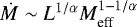 , where Meff= M(1 −Γ) and Γ is the Eddington factor, which for a canonical value of α = 2∕3 (Puls et al. 2000) gives
 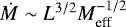 . However, in our approach, all stellar parameters depend on Teff and spectraltype, which may lead to simplification of the relationship. CMF models with base flux taken from hydrostatic atmosphere models (Krtička & Kubát 2012) predict dependence of mass-loss rates on the luminosity class. This dependence disappears in the present models as a result of a stronger reduction of mass-loss rates connected with abandoning of core-hale approximation in spectroscopically less evolved stars.
4 Comparison with observations
4.1 Mass-loss rates
The mass-loss rate determinations for Magellanic Cloud stars are typically based either on the optical spectroscopy (mostly Hα line) or on the UV spectroscopy (P Cygni lines). We collected available recent observational mass-loss rate estimates derived for Magellanic Cloud stars from the optical and UV spectroscopy and plotted them as a function of stellar luminosity in a comparison with our predicted mass-loss rates in Fig. 2. The observational mass-loss rate estimates determined from Hα line (assuming the β-velocity law) are higher possibly as a result of neglected clumping. Consequently, the Hα line alone is not sufficient to determine a precise value of the mass-loss rate (e.g., Puls et al. 2008). On the other hand, although the differences between UV line profiles calculated with and without clumping are rather tiny (Crowther et al. 2002; Evans et al. 2004), precise spectroscopy is able to reveal the influence of clumping on spectra. In the case of mass-loss rates derived from UV spectroscopy, we therefore used only mass-loss rate estimates corrected for clumping. However, these estimates account only for optically thin clumps (microclumping), while a more general approach allows also for optically thick clumps (macroclumping, Oskinova et al. 2007; Sundqvist et al. 2010, 2011; Šurlan et al. 2012, 2013; Shenar et al. 2015; Kubátová et al. 2016).
The mass-loss rates derived from optical spectroscopy are higher on average by a factor of 6.6 than the theoretical predictions for LMC and by a factor of 3.3 for SMC. We also note that the ratio between optical mass-loss rates and theoretical prediction for LMC stars with L ≲ 105 L⊙ is higher than for more luminous stars. This is the main reason why the average ratio is higher for LMC stars than for SMC stars, because the SMC sample contains mostly more luminous stars. On the other hand, the predicted mass-loss rates are consistent with upper limits derived by Mokiem et al. (2007a), Ramírez-Agudelo et al. (2017), and Sabín-Sanjulián et al. (2017). The latter upper limits are not plotted in Fig. 2. As a result of the density squared dependence of recombination rates, the Hα mass-loss rate estimates are sensitive to small-scale inhomogeneities (clumping, e.g., Puls et al. 2006). In the presence of clumping, the Hα mass-loss rates are overestimated by a factor  , where Cc is the clumping factor. The difference between the observational and theoretical mass-loss rates would imply a clumping factor (averaging results for LMC and SMC) Cc = 5.02 = 25 if the difference is purely the result of the influence of clumping on observations. However, clumping also affects the theoretical predictions (Muijres et al. 2011) in the case when clumping starts close to the star. Assuming optically thin inhomogeneities (microclumping) throughout the whole wind, the mass-loss rate scales on average as
  with α ≈ 1∕4 (Muijres et al. 2011, Table 3). Consequently, if the ratio 5.0 between the mass-loss rates is both due to influence of clumping on observations and predictions, then the required clumping factor is only moderate; from
 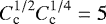 we derive Cc = 9. This would also imply that the true mass-loss rates (i.e., with clumping included in the hydrodynamical models) are by a factor of
  higher than those predicted here. However, if clumping starts above the critical point, where the wind mass-loss rate is estimated, then the difference between observation and theory would imply a relatively large clumping factor, Cc = 25. These results are comparable with that derived for Galactic stars (Krtička & Kubát 2017), who found that Cc ≥ 8. On the other hand, porosity either in the spatial or velocity space may lead to a decrease of the mass-loss rate (Muijres et al. 2011; Sundqvist et al. 2014).
We have demonstrated that the clumping factor is nearly the same in LMC and SMC as in our Galaxy. This agrees with observational studies that also found that the level of clumping does not depend on metallicity (Marchenko et al. 2007; Mokiem et al. 2007b). The observational dependence of mass-loss rate on luminosity in Fig. 2 is wider for low-luminosity (L ≲ 105 L⊙) giants from the sample of Ramírez-Agudelo et al. (2017). This may indicate higher levels of clumping in some of these stars.
The mass-loss rates predicted by our hydrodynamic models either agree with or are slightly higher than mass-loss rates derived by Bouret et al. (2003, 2013, 2015) from UV analysis for high-luminosity (L ≳ 2 × 10⁵ L⊙) SMC stars (see lower panel of Fig. 2). The UV analysis typically accounts for optically thin clumps (microclumping). A more general analysis that accounts also for optically thick clumps (Oskinova et al. 2007; Sundqvist et al. 2011; Šurlan et al. 2013) may explain why some of the predicted mass-loss rates are higher than those derived from observations.
For stars with low luminosity (L ≲ 2 × 10⁵ L⊙), the mass-loss rates derived from UV wind line profiles are significantly lower than the predicted mass-loss rates (Fig. 2, see also Martins et al. 2004). This discrepancy between theory and observations is termed “weak wind problem”. This problem is possibly caused by an overly long shock cooling time, which becomes comparable to the characteristic flow time in low-density environment (Cohen et al. 2008; Krtička & Kubát 2009; Lucy 2012; Huenemoerder et al. 2012). Most of the wind remains hot in such a case and does not leave any imprints in the UV spectra.
Massa et al. (2017) derived mass-loss rates of Magellanic Cloud O stars from mid-infrared excesses. Comparison with our model mass-loss rate shows that our estimates are a factor of 50 lower for SMC stars and a factor of 24 lower for LMC stars. We have not detected any significant luminosity dependence of the difference for SMC stars and increase of the difference with decreasing luminosity for LMC stars. Repeating the same analysis as that done for Hα mass-loss rates, this would imply a clumping factor of at least 120, which is significantly higher than that derived in the Hα formation region. The possibility that the difference is caused by small velocity gradients (suggested by Massa et al. 2017) is not supported by the results of our models.
From the absence of frequency dependence of the observed pulse-arrival times in SMC binary pulsar PSR J0045-7319, Kaspi et al. (1996) derived an upper limit of the B1V star wind mass-loss rate Ṁ < 1.1 × 10⁻¹⁰ M⊙ yr−1 (taking into account the wind terminal velocity derived in Krtička 2014). With luminosity of a B1-type star (Harmanec 1988) we derive from Eq. (1) Ṁ = 3.5 × 10⁻¹⁰ M⊙ yr−1, not far from the observational constraint.
In Fig. 2 we also compared our model results with theoretical predictions of Vink et al. (2001) calculated for giants from Table 1 and metallicities corresponding to LMC and SMC. Because Vink et al. (2001) predictions assume Anders & Grevesse (1989) reference solar abundances, which are higher than those derived by Asplund et al. (2009), we scaled the SMC and LMC abundances by a ratio of the mass-fraction of heavier elements derived by Asplund et al. (2009) and mass-fraction derived by Anders & Grevesse (1989). Our predicted mass-loss rates are typically a factor of 2–3 lower than the predictions of Vink et al. (2001) The difference is lower for SMC stars than for LMC stars and could possibly be attributed to a different method of the calculation of the line force (Krtička & Kubát 2017). While Vink et al. (2001) use the Sobolev method, our models are based on the CMF line force. We derived similar results for Galactic stars (Krtička & Kubát 2017), for which the empirical mass-loss rate estimates corrected for clumping may be reconciled with theoretical predictions in such a way that the average ratio between individual mass-loss rate estimates is not higher than about 1.6.
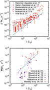 |
Fig. 2 Predicted dependence of the mass-loss rate on luminosity Eq. (1) (solid line) for LMC (upper panel) and SMC (lower panel) in comparison with data derived from optical spectroscopy (red symbols, Massey et al. 2004, 2005; Mokiem et al. 2006, 2007a; Bestenlehner et al. 2014; Ramírez-Agudelo et al. 2017; Sabín-Sanjulián et al. 2017) and UV spectroscopy (violet symbols, Bouret et al. 2003, 2013, 2015). Vertical arrows denote upper limits. The results of Bouret et al. (2015) were derived for stars from IC 1613 and WLM dwarf galaxies, which have a similar metallicity as SMC. Dashed lines denote predictions of Vink et al. (2001) for giants from Table 1. |
4.2 Terminal velocities
According to the predictions of hot-star wind theory, the wind terminal velocity v∞ is proportional to the escape speed vesc (Castor et al. 1975). Although the wind terminal velocity can be readily derived from the observed spectra, the predictions are sensitive to many approximations involved in the calculation of the radiative force, including the treatment of X-rays and clumping. For SMC stars we found the average ratio v∞ ∕vesc = 2.1 and for LMC stars we found the same value as for Galactic stars (Krtička & Kubát 2017) v∞ ∕vesc = 1.9. This is at odds with the findings of Leitherer et al. (1992), who predict v∞ ~ Z0.13 from their theoretical models. Moreover, our predicted ratio v∞∕vesc shows a large scatter and is around 2 for stars with Teff ≳ 32 000 K and increases up to 3 for the coolest stars considered here.
The observational results show large scatter and do not provide a clear clue to the metallicity variations of v∞ . However, contrary to the Galactic O stars (Krtička & Kubát 2017), the theoretical results do not disagree with terminal velocities derived from observations, which give v∞∕vesc = 2.2 ± 0.3 for SMC and v∞∕vesc = 2.6 ± 0.7 for LMC stars (averaging the results of Puls et al. 1996; Crowther et al. 2002; Massey et al. 2005; and Bouret et al. 2013 for 30 000 K ≤ Teff ≤ 45 000 K).
4.3 Ionization fractions
Ionization fractions of some ions can be derived from UV wind line profiles. However, for such an analysis the wind mass-loss rates are required, because the depth of the line profile depends also on the wind density. Moreover, the strength of the line profiles is affected by optically thick inhomogeneities (macroclumping, porosity, Oskinova et al. 2007; Sundqvist et al. 2011; Šurlan et al. 2013). Ionization fractions are furthermore influenced by clumping and X-ray ionization (MacFarlane et al. 1994; Pauldrach et al. 2001; Puls et al. 2006; Carneiro et al. 2016).
Therefore, we selected just the P v ion for the comparison of predicted ionization fractions and ionization fractions derived from observations. The UV lines of this ion are not saturated and this ion is not significantly affected by X-ray ionization (Krtička &Kubát 2012). P v gained considerable attention due to its unexpectedly weak line profiles (Fullerton et al. 2006). The ionization fractions of P v from LMC stars as a function of wind velocity were derived by Massa et al. (2003) using the approximate SEI (Sobolev with exact integration) method. To account for the mass-loss rate dependence of observational indicators, we scaled Massa et al. (2003) ionization fractions by the ratio of the mass-loss rates used to derive these fractions and our predicted mass-loss rates for LMC stars. The comparison of ionization fraction derived from observations and theory is given in Fig 3. The comparison shows that our models are able to reliably reproduce the P v ionization fraction in the winds of LMC stars for stars with Teff≤ 40 000 K. For hotter stars,P vi dominates in the models and the predicted P v ionization fractions are lower than those derived from observations.
 |
Fig. 3 Comparison of predicted P v ionization fractions (blue dots) with ionization fractions derived from observations (Massa et al. 2003, crosses) at the point where the wind velocity is equal to half of its terminal value for LMC stars as a function of stellar effective temperature. The ionization fractions derived from observations were scaled by the ratio of mass-loss rate used to derive the observational fractions and our predicted mass-loss rate for LMC metallicity. |
4.4 Observed spectra
The comparison with observed spectra provides the most detailed test of any model atmosphere. Such comparison is not the aim of the current paper, because some effects that are important for comparison with observations (e.g., clumping and X-rays) are missing in the discussed models. In addition, we calculated a grid of typical models and did not attempt to fit any specific star using our models. However, the emergent spectrum from our models should not be too far away from the observed one.
To demonstrate this, we compared the observed spectra of two stars with one of the models from the grid with parameters close to the studied stars. We selected LMC stars HDE 269698 (Sk -67 166) and HDE 270952 (Sk -65 22) studied by Crowther et al. (2002). We compared the predicted spectra with HST/FOS (HDE 269698, y14m0c05t and y14m0c06t) and IUE (HDE 270952, SWP 1628) observations in Fig. 4. The observations were downloaded and processed using the SPLAT package (Draper 2004; Škoda 2008). The comparison shows that our models are able to predict reasonable wind profiles. However, the photospheric line profiles are not well reproduced, because we focus on wind dynamics and do not include photosphere fully self-consistently. For example, we use the Sobolev approximation to calculate the line source function in kinetic equilibrium equations, which is an oversimplification that may affect the population numbers.
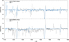 |
Fig. 4 Comparison of predicted LMC 425-1 and 350-1 star spectra with HST/FOS and IUE spectra of stars HDE 269698 and HDE 270952 with parameters close to that of the grid. |
5 Conclusions
We calculated global (unified, hydrodynamic) model atmospheres for a set of model O stars with metallicities corresponding to those in Large and Small Magellanic Clouds. Our models solve CMF radiative transfer, kinetic equilibrium (NLTE), and hydrodynamical equations from (quasi-)hydrostatic atmosphere outwards to expanding stellar wind. Therefore, the models predict the radial variations of density, velocity, and temperature simply from basic global stellar parameters.
As a result of lower metallicity of Magellanic Clouds, the line radiative force is weaker, which leads to lower wind mass-loss rates with respect to the Galactic stars. On average, for Galactic and Magellanic Cloud metallicities the mass-loss rate scales with metallicity as Ṁ ~ Z0.59. We provide a more accurate formula that fits the wind mass-loss rate predicted by our models as a function of stellar luminosity and metallicity.
In comparison with observations, the mass-loss rates following from our hydrodynamic models are lower than mass-loss rates derived from Hα emission line profiles and can be reconciled with Hα diagnostics assuming a clumping factor of Cc = 9. On the other hand, the model mass-loss rates either agree with or are higher than the mass-loss rates derived from UV line profiles. The model P v ionization fractions agree with results derived from observations for LMC stars with Teff≤ 40 000 K. Taken together, our theoretical predictions provide reasonable models with consistent mass-loss rate determination and can be used to study stars from Magellanic Clouds.
Acknowledgements
This work was supported by grant GA ČR 13-10589S. Access to computing and storage facilities owned by parties and projects contributing to the National Grid Infrastructure MetaCentrum provided under the programme “Projects of Large Research, Development, and Innovations Infrastructures” (CESNET LM2015042) is greatly appreciated. The Astronomical Institute Ondřejov is supported by the project RVO:67985815. This research made use of the IUE data derived from the INES database and of the HST data derived from the MAST database using the SPLAT package.
Appendix A Additional figures
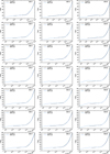 |
Fig. A.1 Comparison of the dependence of temperature on electron density in TLUSTY and METUJE models for SMC stars. The graphs are plotted for individual model stars from Table 1 (denoted in the graphs). |
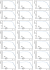 |
Fig. A.2 Comparison of the emergent flux from TLUSTY and METUJE models for SMC stars. The graphs are plotted for individual model stars from Table 1 (denoted in the graphs). |
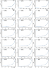 |
Fig. A.3 Comparison of the dependence of temperature on electron density in TLUSTY and METUJE models for LMC stars. The graphs are plotted for individual model stars from Table 1 (denoted in the graphs). |
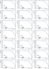 |
Fig. A.4 Comparison of the emergent flux from TLUSTY and METUJE models for LMC stars. The graphs are plotted for individual model stars from Table 1 (denoted in the graphs). |
References
- Abbott, B. P., Abbott, R., Abbott, T. D., et al. 2016, ApJ, 818, L22 [Google Scholar]
- Anders, E., & Grevesse, N. 1989, Geochim. Cosmochim. Acta, 53, 197 [Google Scholar]
- Asplund, M., Grevesse, N., Sauval, A. J., & Scott, P. 2009, ARA&A, 47, 481 [NASA ADS] [CrossRef] [Google Scholar]
- Bestenlehner, J. M., Gräfener, G., Vink, J. S., et al. 2014, A&A, 570, A38 [NASA ADS] [CrossRef] [EDP Sciences] [Google Scholar]
- Bouret, J.-C., Lanz, T., Hillier, D. J., et al. 2003, ApJ, 595, 1182 [NASA ADS] [CrossRef] [Google Scholar]
- Bouret, J.-C., Hillier, D. J., Lanz, T., & Fullerton, A. W. 2012, A&A, 544, A67 [NASA ADS] [CrossRef] [EDP Sciences] [Google Scholar]
- Bouret, J.-C., Lanz, T., Martins, F., et al. 2013, A&A, 555, A1 [NASA ADS] [CrossRef] [EDP Sciences] [Google Scholar]
- Bouret, J.-C., Lanz, T., Hillier, D. J., et al. 2015, MNRAS, 449, 1545 [NASA ADS] [CrossRef] [Google Scholar]
- Carneiro, L. P., Puls, J., Sundqvist, J. O., & Hoffmann, T. L. 2016, A&A, 590, A88 [NASA ADS] [CrossRef] [EDP Sciences] [Google Scholar]
- Castor, J. I., Abbott, D. C., & Klein, R. I. 1975, ApJ, 195, 157 [NASA ADS] [CrossRef] [Google Scholar]
- Cohen, D. H., Kuhn, M. A., Gagné, M., Jensen, E. L. N., & Miller, N. A. 2008, MNRAS, 386, 1855 [NASA ADS] [CrossRef] [Google Scholar]
- Cohen, D. H., Wollman, E. E., Leutenegger, M. A., et al. 2014, MNRAS, 439, 908 [NASA ADS] [CrossRef] [Google Scholar]
- Crowther, P. A., Hillier, D. J., Evans, C. J., et al. 2002, ApJ, 579, 774 [NASA ADS] [CrossRef] [Google Scholar]
- Draper, P. W. 2004, SPLAT: A Spectral Analysis Tool, Starlink User Note 243 (University of Durham) [Google Scholar]
- Evans, C. J., Crowther, P. A., Fullerton, A. W., & Hillier, D. J. 2004, ApJ, 610, 1021 [NASA ADS] [CrossRef] [Google Scholar]
- Fullerton, A. W., Massa, D. L., Prinja, R. K. 2006, ApJ, 637, 1025 [NASA ADS] [CrossRef] [Google Scholar]
- Gräfener, G. 2003, in Stellar Atmosphere Modeling, ASP Conf. Proc., 288, 533 [NASA ADS] [Google Scholar]
- Gräfener, G., & Hamann, W.-R. 2008, A&A, 482, 945 [NASA ADS] [CrossRef] [EDP Sciences] [Google Scholar]
- Harmanec, P. 1988, Bull. Astr. Inst. Czechosl. 39, 329 [Google Scholar]
- Herrero, A., Garcia, M., Puls, J., et al. 2012, A&A, 543, A85 [NASA ADS] [CrossRef] [EDP Sciences] [Google Scholar]
- Hill, V., Andrievsky, S., & Spite, M. 1995, A&A, 293, 347 [NASA ADS] [Google Scholar]
- Huenemoerder, D. P., Oskinova, L. M., Ignace, R., et al. 2012, ApJ, 756, L34 [NASA ADS] [CrossRef] [Google Scholar]
- Hummer, D. G., Berrington, K. A., Eissner, W., et al. 1993, A&A, 279, 298 [NASA ADS] [Google Scholar]
- Kaspi, V. M., Tauris, T. M., & Manchester, R. N. 1996, ApJ, 459, 717 [NASA ADS] [CrossRef] [Google Scholar]
- Keszthelyi, Z., Puls, J., & Wade, G. A. 2017, A&A, 598, A4 [NASA ADS] [CrossRef] [EDP Sciences] [Google Scholar]
- Kramida, A., Ralchenko, Y., Reader, J., & NIST ASD Team 2015, NIST Atomic Spectra Database (version 5.2) (Gaithersburg, MD: National Institute of Standards and Technology) [Google Scholar]
- Krtička, J. 2006, MNRAS, 367, 1282 [NASA ADS] [CrossRef] [Google Scholar]
- Krtička, J. 2014, A&A, 564, A70 [Google Scholar]
- Krtička, J., & Kubát, J. 2006, A&A, 446, 1039 [NASA ADS] [CrossRef] [EDP Sciences] [Google Scholar]
- Krtička, J., & Kubát, J. 2009, MNRAS, 394, 2065 [NASA ADS] [CrossRef] [Google Scholar]
- Krtička, J., & Kubát, J. 2010, A&A, 519, A5 [NASA ADS] [CrossRef] [EDP Sciences] [Google Scholar]
- Krtička, J., & Kubát, J. 2012, MNRAS, 427, 84 [NASA ADS] [CrossRef] [Google Scholar]
- Krtička, J., & Kubát, J. 2017, A&A, 606, A31 [NASA ADS] [CrossRef] [EDP Sciences] [Google Scholar]
- Kubát, J. 1996, A&A, 305, 255 [NASA ADS] [Google Scholar]
- Kubát, J., Puls, J., & Pauldrach, A. W. A. 1999, A&A, 341, 587 [NASA ADS] [Google Scholar]
- Kubátová, B., Hamann, W.-R., Todt, H., et al. 2016, in Wolf-Rayet Stars, eds. W.-R. Hamann, A. Sander, & H. Todt (Universitätsverlag Potsdam), 125 [Google Scholar]
- Kupka, F., Piskunov, N. E., Ryabchikova, T. A., Stempels, H. C., & Weiss, W. W. 1999, A&AS, 138, 119 [NASA ADS] [CrossRef] [EDP Sciences] [MathSciNet] [PubMed] [Google Scholar]
- Lanz, T., & Hubeny, I. 2003, ApJS, 146, 417 [NASA ADS] [CrossRef] [Google Scholar]
- Lanz, T., & Hubeny, I. 2007, ApJS, 169, 83 [CrossRef] [Google Scholar]
- Leitherer, C., Robert, C., & Drissen, L. 1992, ApJ, 401, 596 [NASA ADS] [CrossRef] [Google Scholar]
- Lucy, L. B. 2012, A&A, 544, A120 [NASA ADS] [CrossRef] [EDP Sciences] [Google Scholar]
- MacFarlane, J. J., Cohen, D. H., & Wang, P. 1994, ApJ, 437, 351 [NASA ADS] [CrossRef] [Google Scholar]
- Marchenko, S. V., Foellmi, C., Moffat, A. F. J., et al. 2007, ApJ, 656, L77 [NASA ADS] [CrossRef] [Google Scholar]
- Martins, F., Schaerer, D., Hillier, D. J., & Heydari-Malayeri, M. 2004, A&A, 420, 1087 [NASA ADS] [CrossRef] [EDP Sciences] [Google Scholar]
- Martins, F., Schaerer, D., & Hillier, D. J. 2005, A&A, 436, 1049 [NASA ADS] [CrossRef] [EDP Sciences] [Google Scholar]
- Massa, D., Fullerton, A. W., Sonneborn, G., Hutchings, J. B. 2003, ApJ, 586, 996 [NASA ADS] [CrossRef] [Google Scholar]
- Massa, D., Fullerton, A. W., & Prinja, R. K. 2017, MNRAS, 470, 3765 [NASA ADS] [CrossRef] [Google Scholar]
- Massey, P., Bresolin, F., Kudritzki, R. P., Puls, J., & Pauldrach, A. W. A. 2004, ApJ, 608, 1001 [Google Scholar]
- Massey, P., Puls, J., Pauldrach, A. W. A., et al. 2005, ApJ, 627, 477 [NASA ADS] [CrossRef] [Google Scholar]
- Mihalas, D., Kunasz, P. B., & Hummer, D. G. 1975, ApJ, 202, 465 [NASA ADS] [CrossRef] [Google Scholar]
- Mokiem, M. R., de Koter, A., Evans, C. J., et al. 2006, A&A, 456, 1131 [NASA ADS] [CrossRef] [EDP Sciences] [Google Scholar]
- Mokiem, M. R., de Koter, A., Evans, C. J., et al. 2007a, A&A, 465, 1003 [NASA ADS] [CrossRef] [EDP Sciences] [Google Scholar]
- Mokiem, M. R., de Koter, A., Vink, J. S., et al. 2007b, A&A, 473, 603 [NASA ADS] [CrossRef] [EDP Sciences] [Google Scholar]
- Muijres, L., de Koter, A., Vink, J., et al. 2011, A&A, 526, A32 [Google Scholar]
- Najarro, F., Hanson, M. M., & Puls, J. 2011, A&A, 535, A32 [NASA ADS] [CrossRef] [EDP Sciences] [Google Scholar]
- Oskinova, L. M., Hamann, W.-R., & Feldmeier, A. 2007, A&A, 476, 1331 [NASA ADS] [CrossRef] [EDP Sciences] [Google Scholar]
- Pauldrach, A. W. A., Hoffmann, T. L., & Lennon, M. 2001, A&A, 375, 161 [NASA ADS] [CrossRef] [EDP Sciences] [Google Scholar]
- Pauldrach, A. W. A., Vanbeveren, D., & Hoffmann, T. L., 2012, A&A, 538, A75 [NASA ADS] [CrossRef] [EDP Sciences] [Google Scholar]
- Petrov, B., Vink, J. S., & Gräfener, G. 2016, MNRAS, 458, 1999 [NASA ADS] [CrossRef] [Google Scholar]
- Piskunov, N. E., Kupka, F., Ryabchikova, T. A., Weiss, W. W., & Jeffery, C. S. 1995, A&AS, 112, 525 [NASA ADS] [Google Scholar]
- Puebla, R. E., Hillier, D. J., Zsargó, J., Cohen, D. H., & Leutenegger, M. A. 2016, MNRAS, 456, 2907 [NASA ADS] [CrossRef] [Google Scholar]
- Puls, J., Kudritzki, R.-P., Herrero, A., et al. 1996, A&A, 305, 171 [NASA ADS] [Google Scholar]
- Puls, J., Springmann, U., & Lennon, M. 2000, A&AS, 141, 23 [NASA ADS] [CrossRef] [EDP Sciences] [Google Scholar]
- Puls, J., Markova, N., Scuderi, S., et al., 2006, A&A, 454, 625 [NASA ADS] [CrossRef] [EDP Sciences] [Google Scholar]
- Puls, J., Markova, N., & Scuderi, S. 2008, in Mass Loss from Stars and the Evolution of Stellar Clusters, eds. A. de Koter, L. Smith, & R. Waters (San Francisco: ASP), 101 [Google Scholar]
- Ramírez-Agudelo, O. H., Sana, H., de Koter, A., et al. 2017, A&A, 600, A81 [NASA ADS] [CrossRef] [EDP Sciences] [Google Scholar]
- Rauw, G., Hervé, A., Nazé, Y., et al. 2015, A&A, 580, A59 [NASA ADS] [CrossRef] [EDP Sciences] [Google Scholar]
- Rolleston, W. R. J., Trundle, C., & Dufton, P. L. 2002, A&A, 396, 53 [NASA ADS] [CrossRef] [EDP Sciences] [Google Scholar]
- Sabín-Sanjulián, C., Simón-Díaz, S., Herrero, A., et al. 2017, A&A, 601, A79 [NASA ADS] [CrossRef] [EDP Sciences] [Google Scholar]
- Sander, A. A. C., Hamann, W.-R., Todt, H., Hainich, R., & Shenar, T. 2017, A&A, 603, A86 [NASA ADS] [CrossRef] [EDP Sciences] [Google Scholar]
- Seaton, M. J., Zeippen, C. J., Tully, J. A., et al. 1992, Rev. Mex. Astron. Astrofis., 23, 19 [NASA ADS] [EDP Sciences] [Google Scholar]
- Shenar, T., Oskinova, L., Hamann, W.-R., et al. 2015, ApJ, 809, 135 [NASA ADS] [CrossRef] [Google Scholar]
- Škoda, P. 2008, in Astronomical Spectroscopy and Virtual Observatory Proc., eds. M. Guainazzi, & P. Osuna, (ESA), 97 [Google Scholar]
- Sundqvist, J. O., Puls, J., & Feldmeier, A. 2010, A&A, 510, A11 [NASA ADS] [CrossRef] [EDP Sciences] [Google Scholar]
- Sundqvist, J. O., Puls, J., Feldmeier, A., Owocki, S. P. 2011, A&A, 528, A6 [Google Scholar]
- Sundqvist, J. O., Puls, J., & Owocki, S. P. 2014, A&A, 568, A59 [NASA ADS] [CrossRef] [EDP Sciences] [Google Scholar]
- Šurlan, B., Hamann, W.-R., Kubát, J., Oskinova, L., & Feldmeier, A. 2012, A&A, 541, A37 [NASA ADS] [CrossRef] [EDP Sciences] [Google Scholar]
- Šurlan, B., Hamann, W.-R., Aret, A., et al. 2013, A&A, 559, A130 [NASA ADS] [CrossRef] [EDP Sciences] [Google Scholar]
- Tramper, F., Sana, H., de Koter, A., & Kaper, L. 2011, ApJ, 741, L8 [NASA ADS] [CrossRef] [Google Scholar]
- Venn, K. A. 1999, ApJ, 518, 405 [NASA ADS] [CrossRef] [Google Scholar]
- Vink, J. S., de Koter, A., & Lamers, H. J. G. L. M. 2001, A&A, 369, 574 [NASA ADS] [CrossRef] [EDP Sciences] [Google Scholar]
All Tables
Stellar parameters of the model grid with derived values of the terminal velocity v∞ and mass-lossrate Ṁ.
All Figures
|
Fig. 1 Convergence of the hydrodynamical structure of the LMC 400-3 model. Left plot: maximum relative difference between hydrodynamical variables in subsequent iteration steps as a function of total number of hydrodynamical iterations. We note that kinetic equilibrium equations are iterated for each step of hydrodynamical iterations. Blue vertical strips denote a new step of a global iteration (numbered in the bottom of the plot) when the inner boundary velocity (and the mass-loss rate) is changed. Labels a–d in the bottom of the plot indicate (see also Krtička & Kubát 2017, Sect. 2): Panel a:calculation of the initial model for subcritical velocities. In the first few steps the CMF radiative transfer is not solved. Afterwards, the CMF calculations are switched on (indicated by a blue arrow). Panel b: iteration of wind model with mass-loss rate lower than or equal to the final one. Each model denoted as b has a higher mass-loss rate than the previous one. Panel c: iteration of wind model with mass-loss rate lower than the final one and inclusion of model for supercritical velocities. Here the blue arrow denotes inclusion of model for supercritical velocities. Panel d: iteration of wind model with mass-loss rate higher than the final one. After this step the model mass-loss rate decreases. The plot shows that the convergence of hydrodynamical structure in each step is stable and relatively fast. Right plot: mass-loss rate in individual global iteration steps (numbers on horizontal axis are the same as in blue labels in the left plot). The models converge to a final mass-loss rate given in Table 1. |
| In the text | |
|
Fig. 2 Predicted dependence of the mass-loss rate on luminosity Eq. (1) (solid line) for LMC (upper panel) and SMC (lower panel) in comparison with data derived from optical spectroscopy (red symbols, Massey et al. 2004, 2005; Mokiem et al. 2006, 2007a; Bestenlehner et al. 2014; Ramírez-Agudelo et al. 2017; Sabín-Sanjulián et al. 2017) and UV spectroscopy (violet symbols, Bouret et al. 2003, 2013, 2015). Vertical arrows denote upper limits. The results of Bouret et al. (2015) were derived for stars from IC 1613 and WLM dwarf galaxies, which have a similar metallicity as SMC. Dashed lines denote predictions of Vink et al. (2001) for giants from Table 1. |
| In the text | |
|
Fig. 3 Comparison of predicted P v ionization fractions (blue dots) with ionization fractions derived from observations (Massa et al. 2003, crosses) at the point where the wind velocity is equal to half of its terminal value for LMC stars as a function of stellar effective temperature. The ionization fractions derived from observations were scaled by the ratio of mass-loss rate used to derive the observational fractions and our predicted mass-loss rate for LMC metallicity. |
| In the text | |
|
Fig. 4 Comparison of predicted LMC 425-1 and 350-1 star spectra with HST/FOS and IUE spectra of stars HDE 269698 and HDE 270952 with parameters close to that of the grid. |
| In the text | |
|
Fig. A.1 Comparison of the dependence of temperature on electron density in TLUSTY and METUJE models for SMC stars. The graphs are plotted for individual model stars from Table 1 (denoted in the graphs). |
| In the text | |
|
Fig. A.2 Comparison of the emergent flux from TLUSTY and METUJE models for SMC stars. The graphs are plotted for individual model stars from Table 1 (denoted in the graphs). |
| In the text | |
|
Fig. A.3 Comparison of the dependence of temperature on electron density in TLUSTY and METUJE models for LMC stars. The graphs are plotted for individual model stars from Table 1 (denoted in the graphs). |
| In the text | |
|
Fig. A.4 Comparison of the emergent flux from TLUSTY and METUJE models for LMC stars. The graphs are plotted for individual model stars from Table 1 (denoted in the graphs). |
| In the text | |
Current usage metrics show cumulative count of Article Views (full-text article views including HTML views, PDF and ePub downloads, according to the available data) and Abstracts Views on Vision4Press platform.
Data correspond to usage on the plateform after 2015. The current usage metrics is available 48-96 hours after online publication and is updated daily on week days.
Initial download of the metrics may take a while.