| Issue |
A&A
Volume 564, April 2014
|
|
|---|---|---|
| Article Number | A132 | |
| Number of page(s) | 10 | |
| Section | The Sun | |
| DOI | https://doi.org/10.1051/0004-6361/201322886 | |
| Published online | 17 April 2014 | |
On the formation of Mg ii h and k lines in solar prominences
1
Astronomical Institute, Academy of Sciences of the Czech
Republic,
25165
Ondřejov,
Czech Republic
e-mail:
pheinzel@asu.cas.cz
2
Max-Planck-Institut für Astrophysik, Karl-Schwarzschild-Str. 1, 85740
Garching,
Germany
3
Institut d’Astrophysique Spatiale, Université Paris XI/CNRS,
91405
Orsay Cedex,
France
Received:
21
October
2013
Accepted:
23
January
2014
Aims. With the recent launch of the IRIS mission, it has become urgent to develop the spectral diagnostics using the Mg ii resonance h and k lines. In this paper, we aim to demonstrate the behavior of these lines under various prominence conditions. Our results serve as a basis for analysis of new IRIS data and for more sophisticated prominence modeling.
Methods. For this exploratory work, we use a canonical 1D prominence-slab model, which is isobaric and may have three different temperature structures: isothermal, PCTR-like (prominence-corona transition region), and consistent with the radiative equilibrium. The slabs are illuminated by a realistic incident solar radiation obtained from the UV observations. A five-level plus continuum Mg ii model atom is used to solve the full NLTE problem of the radiative transfer. We use the numerical code based on the ALI techniques and apply the partial frequency redistribution for both Mg ii resonance lines. We also use the velocity-dependent boundary conditions to study the effect of Doppler dimming in the case of moving prominences. Finally, the relaxation technique is used to compute a grid of models in radiative equilibrium.
Results. We computed the Mg ii h and k line profiles that are emergent from prominence-slab models and show their dependence on kinetic temperature, gas pressure, geometrical extension, and microturbulent velocity. By increasing the line opacity, significant departures from the complete frequency redistribution take place in the line wings. Models with a PCTR temperature structure show that Mg ii becomes ionized to Mg iii in the temperature range between roughly 15 000 and 30 000 K. Doppler dimming is significant for Mg ii resonance lines. At the velocity 300 km s-1, the line intensity decreases to about 20% of the value for static prominences. Finally, we demonstrate the role of Mg ii h and k radiation losses on the prominence energy balance. Their dominant role is at lower pressures, while the losses due to hydrogen and Ca ii dominate at higher pressures.
Key words: line: profiles / line: formation / Sun: filaments, prominences
© ESO, 2014
1. Introduction
The solar UV resonance lines of Mg ii at 2795.53 (k) and 2802.71 (h) Å (in the air wavelengths), are only accessible from space, whether from a balloon or spacecraft. As for the Ca ii lines, they are commonly considered as chromospheric indicators of activity, and the two lines have been coined h and k, similarly to the H and K lines of Ca ii. With space UV instrumentation, it was possible to record (or at least to detect) Mg ii h and k lines in various structures, including a prominence (Bonnet et al. 1967), but the spectral resolution was insufficient for recording a profile. During a balloon flight, Lemaire & Skumanich (1973) not only obtained high spectral resolution (2.5 pm = 0.025 Å) observations and evidenced strong self-reversals (a solid proof that the h and k lines are optically thick) but also performed a NLTE modeling of the solar chromosphere, which was already initiated by Skumanich (1967). Here NLTE stands for departures from a local thermodynamic equilibrium (LTE). Later on, the spectral resolution (12 pm) of the NRL spectrograph on SKYLAB also enabled Doschek & Feldman (1977) to show very different reversed profiles in quiet and active areas. With the LPSP polychromator on OSO 8, systematic measurements of the Mg ii profiles have been performed on a large variety of solar structures ranging from the quiet and active Sun (Artzner et al. 1978; Lemaire et al. 1981) to flares (Lemaire et al. 1984). Another nice example was provided by Lites & Skumanich (1982), who took full use of the Mg ii h and k observations for modeling a solar sunspot. Later on, high spectral resolution (1.5 pm) profiles have been obtained by Staath & Lemaire (1995) at the disk center and at the limb. For a recent work on chromospheric modeling using the Mg ii lines, see Leenaarts et al. (2013a,b), Pereira et al. (2013) and Avrett et al. (2013) who discuss the formation of Mg ii lines in the solar atmosphere in detail.
The above mentioned results clearly show that the Mg ii doublet is an excellent tool for the diagnostics of cool plasmas in solar structures, including prominences which consist of the cool material suspended in the hot corona (Tandberg-Hanssen 1995; Labrosse et al. 2010). This was first confirmed by the long-exposure image taken on an out-of-limb prominence (Fredga 1969) and by the spectra of Bonnet et al. (1967). The first high-resolution spectra of the Mg ii doublet (along with Lyman α and Ca ii H and K) in an active region prominence were obtained with the LPSP UV Polychromator on OSO 8 (Vial et al. 1979). The spatial and spectral resolutions were, respectively, 1 × 10 arcsec (i.e., signal integrated along the slit) and 2 pm. The profiles showed an important spatial variability, a line-of-sight (LOS) velocity of about 20 km s-1. The k to h intensity ratio was close to 2. On the contrary, quiescent prominence profiles, which are obtained with a 1 × 20 arcsec resolution, showed unreversed k and h profiles. The k to h ratio was found to be about 1.7, and the derived opacities were about 2.3 for k and 1.2 for h (Vial 1982a).
On the basis of the code for two-dimensional (2D) NLTE modeling of illuminated structures (Mihalas et al. 1998), Vial (1982b) could implement realistic model conditions (ionization degree and shapes of the incident h and k line profiles) and derived some general properties of the lines emerging from the 2D free-standing slabs. For most computed models, the emergent profiles were reversed, except at the top edges of the 2D slab or when radial velocities as small as 20 km s-1 were included. Model and observed parameters were compared in his Table 4. A major finding was that the match between the Mg ii h and k lines, and also hydrogen Lyman α and Ca ii lines required low electron densities (about 2 × 1010 cm-3), as confirmed later on by Bommier et al. (1986), and a relatively low ionization degree of hydrogen. These results, obtained in the so-called complete frequency redistribution (CRD) approximation, were confirmed and improved using the partial frequency redistribution (PRD) approach by Paletou et al. (1993) who also considered 2D models of uniform prominence slabs. Since then, no major work concerning the h and k Mg ii lines in prominences has been performed.
Some very important results concerning filamentation, flows, and waves have been recently obtained in the Ca ii H line with the very high resolution of the Hinode/SOT instrument (e.g. Berger et al. 2008). With the recently launched Interface Region Imaging Spectrograph (IRIS) (De Pontieu et al. 2014, see also http://iris.lmsal.com/), which performs high spatial (0.33 arcsec) and spectral (~50 mÅ) resolution imaging spectroscopy in the h and k lines of Mg ii, we are provided with much needed information on the thermodynamic properties and the full velocity vector of the observed prominences, their fine structures, and prominence-corona transition regions (PCTRs). In Fig. 1, we show an example of the IRIS first-light prominence observations in the Mg ii doublet, which demonstrate very narrow profiles, certain spatial variability, and some Doppler shifts typical for a quiescent prominence. A systematic modeling effort that implies the NLTE radiative transfer is necessary, which is the aim of the present paper.
As mentioned above, 2D prominence models have been used to compute the synthetic profiles of Mg ii lines. However, only large-scale 2D slabs (isothermal with prescribed uniform electron density), representing the whole prominence, have been considered. On the other hand, more complex 2D techniques have been applied to study the behavior of prominences with multithread fine structures in magneto-hydrostatic equilibrium. The resulting hydrogen Lyman spectra were found to be consistent with the SOHO/SUMER observations (Gunár et al. 2008; Gunár 2013, and the references therein). It is our ultimate goal to extend such multithread modeling to other species like calcium, magnesium, and helium. However, we first want to investigate how the realistic range of prominence physical conditions (in both cool central parts and PCTR) will influence the properties of Mg ii lines. In other words, we want to explore a grid of models similar to that of Gouttebroze et al. (1993, hereafter referred to as GHV) and obtain a range of predicted line intensities (profiles and integrated intensities), optical thicknesses, source functions, ionization degrees etc. For this purpose, we use relatively simple 1D models in this study and concentrate on details of the Mg ii line-formation in a multilevel atom with the continuum, using the angle-averaged PRD and extending previously considered isothermal slabs to slabs having PCTR. Note that only a two-level atom without continuum was so far considered in dealing with Mg ii resonance lines in prominences.
The paper is organized as follows: Sect. 2 describes our model and techniques used to compute the synthetic Mg ii line spectra; Sect. 3 provides information about the grid of models used, Sect. 4 shows the results of our synthesis for static prominence models, while Sect. 5 deals with moving (eruptive) prominences. In Sect. 6, we construct the thermal models in radiative equilibrium by adding the magnesium radiative losses to those previously considered by Heinzel & Anzer (2012). Section 7 contains Discussion and Conclusions.
2. Model description
The prominence structure considered in this paper is modeled by one-dimensional (1D) plasma
slabs standing vertically on the solar surface and illuminated by the surrounding quiet
solar atmosphere. We use two types of models: isothermal-isobaric models (as in GHV) and
models with a PCTR, where the isobaric slabs have the temperature structure of the form (see
Anzer & Heinzel 1999),
 (1)Here
Tc
and Tb are the central and boundary
temperatures, respectively, D is the geometrical thickness of the 1D slab, and
x is the
coordinate across the slab. The parameter γtr characterizes the temperature gradient
in models with PCTR.
(1)Here
Tc
and Tb are the central and boundary
temperatures, respectively, D is the geometrical thickness of the 1D slab, and
x is the
coordinate across the slab. The parameter γtr characterizes the temperature gradient
in models with PCTR.
The NLTE modeling is done in two steps. First, we compute the statistical equilibrium for a five-level plus continuum hydrogen atom, to determine the electron densities at all depths; here we neglect the helium ionization. The resulting atmospheric structure is then used to solve the NLTE problem for magnesium. We use the MALI technique (Rybicki & Hummer 1991; Heinzel 1995), with partial redistribution (PRD) in resonance lines (Paletou 1995). The same method was also used for the Ca ii line modeling (see Gouttebroze & Heinzel 2002). The PRD is treated as a standard two-level partial redistribution applicable to strong resonance lines.
In this exploratory study, we use a five-level plus continuum Mg ii-Mg iii model atom to be able to directly apply our MALI-based code, previously used and well tested for the calcium case with PRD. Apart from the two strong h and k resonance lines, we also include three line transitions between the 3P and 3D states. These subordinate lines appear just close to the h and k lines (2790.8, 2797.9 and 2798.0 Å) and are detected in absorption in the chromospheric spectra in the wings of the resonance lines. However, they are very weak and relatively far from h and k lines. As noticed by Milkey & Mihalas (1974) (with the reference to Dumont 1967a), these and other subordinate lines have a negligible effect on the source function of the resonance lines, and we thus neglect other line transitions to 4S state and to higher states. For the Mg ii-Mg iii level diagram, see Leenaarts et al. (2013a), where the same air wavelengths are used. What is really new in the present study of prominences is the self-consistent modeling of Mg ii to Mg iii ionization (only two-level Mg ii atoms without continuum were treated for prominences until now), which is important in PCTR regions where the degree of Mg ii ionization is increasing.
The ionization energies, photoionization cross-sections and the line oscillator strengths are those used by Uitenbroek (1997) and in the PANDORA code (E. Avrett, priv. comm.). Bound-bound collisions with free electrons are treated using the data from Sigut & Pradhan (1995), for collisional ionization we use the data from PANDORA. We neglect collisions with the neutral hydrogen. For the electron Stark broadening of the upper levels of h and k transitions we use the elastic collisional rate given by Milkey & Mihalas (1974). For the magnesium abundance, we use the value 3.5 × 10⁻⁵ given by Vial (1982b). This value is very close to some recent determinations.
In the case of solar prominences, a critical ingredient of any transfer modeling is the incident radiation coming from the surrounding solar atmosphere. For Mg ii transitions, including five continua, we use the following data: the h and k resonance lines as detected on the solar disk with high spectral resolution by the RASOLBA balloon experiment (Staath & Lemaire 1995) and calibrated to absolute units on the basis of the earlier OSO 8 LPSP observations (the ratio between chromospheric line-center k and h intensities we use is 1.25). We neglect any center-to-limb variations here. For subordinate lines, we use the h and k wing intensities at the position of these lines.
The integration over all incident rays for a given height H of the prominence above the solar surface is performed according to Heinzel (1983). This gives the mean intensity of radiation incident on 1D slab models. To compute Mg ii photoionization rates in the five continua, we use the internal continuum radiation field, which is dominated by the hydrogen Lyman continuum below 912 Å, and is prescribed by external UV disk radiation above 912 Å. We also include the hydrogen Lyman lines in the photoionization rates in the same way as in the Ca ii model, where it proved to be very important (see Gouttebroze & Heinzel 2002). Both the Lyman-continuum and Lyman-line radiation fields (depth-dependent) are precomputed in the first step, when the NLTE hydrogen problem is solved.
3. Grid of 1D slab models
In this study, we use a small grid of representative 1D-slab models, which are isobaric and have either an isothermal structure like the GHV models or a PCTR similar to that introduced by Anzer & Heinzel (1999). We neglect here the effect of the magneto-hydrostatic equilibrium and use representative isobaric slabs. In the PCTR case, the temperature distribution takes a semi-empirical form given by Eq. (1). We use a constant microturbulent velocity of 5 km s-1, but we explore models with other values as well. The modeling is made for the prominence height above the solar surface H = 10 000 km, as in GHV. In Table 1, we give the values of the prominence parameters for the studied models.
Grid of 1D-slab models used in this study.
 |
Fig. 1 Uncalibrated stigmatic spectra of the Mg ii k (2795.53 Å) and h (2802.71 Å) lines detected by IRIS at 16:48:59 on July 18, 2013. The upper part of the figure, where the profiles are narrow, corresponds to a prominence seen above the South Pole limb. The lower part of the figure, where profiles are wide and reversed, corresponds to the chromosphere close to (and just above) the limb. The spectrum starts (left) at 2792.78 Å and ends (right) at 2805.34 Å. The spatial extension is 85 arcsec (Courtesy A. Title − LMSAL). |
4. Results for grid models
Using the NLTE radiative-transfer approach described above, we have computed the Mg ii h and k synthetic spectra normally emergent from 1D slabs listed in Table 1. If not indicated otherwise, all profiles were computed using the PRD approach. Since no macroscopic velocity fields were considered in this section, the line profiles are symmetrical with respect to the line center.
4.1. Mg II line profiles emergent from isothermal-isobaric slabs
To explore the diagnostics potential of Mg ii resonance lines, we plot the Mg ii k line profiles normally emergent from our isothermal-isobaric 1D slabs in Figs. 2−4. While the results for D = 200 or even 1000 km may represent cases corresponding to prominence fine-structure elements, D = 5000 km shows the situation when the whole prominence volume (slab) is densely filled by emitting plasma. The individual profiles exhibit the following trends.
Theoretical Mg ii h and k line parameters for 1D isothermal-isobaric prominence slabs.
Both h and k lines show a very similar behavior, which can be also seen from the observed IRIS spectra in Fig. 1. This is why we show only the k-line profiles, but see also Table 2. Their intensities generally increase with the temperature and the gas pressure, which is best visible for p = 0.1 and 0.5 dyne cm-2 and larger geometrical thicknesses. The line reversal has a similar behavior. For the lowest pressure, the line source function S is almost uniform through the slab and only weakly depends on temperature. For such a case, the profiles in the line core are either non-reversed or have a flat plateau since the intensity takes approximately the form I = S(1 − e− τ), where τ is the optical thickness. For higher pressures and thicknesses, the source function starts to decrease toward the slab boundaries and thus the line profiles are reversed. The full width at half maximum (FWHM) also increases with the gas pressure and thickness due to the increase of the optical thickness and will be even larger for viewing directions other than the normal one. Both lines can reach rather large optical thicknesses in the line center up to 103 − 104 for the densest and thickest models. Note that τk/τh = 2 due to the ratio between the statistical weights of the corresponding upper levels. The integrated-intensity ratio is also around two for the thinest models.
For optically-thick models at lower pressures, the k line-center intensities are saturated to values of 2 − 3×10⁻⁷ erg s-1 cm-2 sr-1 Hz-1, which is roughly at the level of the diluted incident radiation. This is not surprising because Mg ii h and k lines are strong resonance lines, and their behavior is similar to that of hydrogen Lyman α (see Heinzel et al. 1987). However, when the temperature and pressure increase, the line-center intensity also increases which reflects the thermal contribution to the otherwise scattering-dominated source function, which strongly departs from the LTE. For optically-thinner models with low pressure and small thickness (see Fig. 2), the central intensities on the other hand lie below this limit, and this might be the observed case mentioned in the introduction. The results of our profile computations generally agree with previous modeling of isobaric-isothermal slabs (Vial 1982b; Paletou et al. 1993− see below), where just the two-level approximation without continuum was used. It follows from our modeling that the line reversals are present only for higher pressures and temperatures (assuming a given geometrical thickness of the structure) but they will be lowered by convolving synthetic profiles with the instrumental profile of the IRIS spectrograph, which has the width on the order of 50 mÅ.
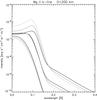 |
Fig. 2 Mg ii k line profiles of the normally emergent radiation from slabs with D = 200 km. The three sets of curves, increasing in their intensity, correspond to three gas pressures p = 0.01, 0.1, and 0.5 dyne cm-2. The gray scale corresponds to three temperatures: T = 6000 K (black), 8000 K (dark gray), and 10 000 K (light gray). Only one half of the symmetrical profiles is displayed. |
In Fig. 5, we demonstrate the sensitivity of Mg ii line profiles to the microturbulence. Microturbulent velocities vt in central cool parts of prominences (which we model in this section) are reported to amount to 3−8 km s-1 (Engvold et al. 1990). For the models used in Figs. 2−4, we set vt = 5 km s-1, but we show a significant increase of the line broadening with increasing vt from zero to 8 km s-1 in Fig. 5. Contrary to hydrogen lines, which are mostly sensitive to thermal broadening that depends on temperature, the metallic lines are known to be very sensitive to the microturbulent broadening and practically insensitive to the thermal one. Assuming Gaussian line profiles for both thermal and microturbulent (nonthermal) broadenings, the resulting Doppler width of Mg ii lines is dominated by the microturbulence. For example, we used three values of T = 6000, 8000, and 10 000 K with vt = 5 km s-1 in our isobaric models and this temperature range leads to an increase in Doppler width of less than 5%. Therefore, the temperature broadening is small, while the nonthermal one is important, as our results in Fig. 5 show. Significant nonthermal broadening of the line absorption profile also leads to an enhanced amount of the absorbed incident radiation. This is due to a sharp increase of the intensity of the incident radiation in both h and k lines in their cores where the dominant contribution to absorption takes place. We can call this effect as “turbulent Doppler brightening” according to Heinzel & Rompolt (1987) (see also Sect. 5). This brightening is clearly visible in Fig. 5.
 |
Fig. 5 Mg ii k line profiles of the normally emergent radiation from the slab with D = 1000 km and T = 8000 K. The two sets of curves correspond to values of the gas pressure p = 0.01 and 0.1 dyne cm-2. For each pressure, three curves show an increasing line broadening for the three values of the microturbulent velocity: 0 km s-1 (black), 3 km s-1 (dark gray), and 8 km s-1 (light gray). |
4.2. Mg II line parameters for isothermal-isobaric models
In this subsection, we present a summary table (Table 2) of the theoretical line parameters for all isothermal-isobaric models from Table 1. The integrated intensities and the peak-to-center ratios have been computed for line profiles displayed in Figs. 2−4 (note that the integrated intensities correspond to the whole symmetrical profiles). Table 2 clearly shows how these parameters vary with the gas pressure, temperature, and geometrical thickness of the prominence slabs and, thus, can provide a rough estimate of the plasma parameters using new data from IRIS. The line reversals, depending on the optical thickness, can be recognized from the observed spectral profiles, without having an absolute intensity calibration. It is worth noting that the Mg ii lines are optically thick in most cases with the line-center optical thickness reaching values between 103 and 104 for our extremal models. The optical thickness increases with increasing gas pressure (and of course with geometrical thickness) but decreases with increasing temperature. The integrated intensity decreases with increasing temperature for the lowest pressure but increases for highest one.
We can also compare our results with those of Paletou et al. (1993), who considered a similar prominence model. They used a 2D slab to model the whole prominence with its height extension of 30 000 km and the line-of-sight thickness of 5000 km. Our 1D slab approximates this extended 2D slab in its middle parts. Paletou et al. (1993) present only one specific model of an isothermal slab, which has the temperature T = 8000 K, constant electron density 2 × 1010 cm-3, and the microturbulent velocity 8 km s-1. With a fixed ionization degree of hydrogen, they obtain the corresponding gas pressure p = 5.15 × 10⁻² dyne cm-2. The center of their 2D slab is located at height 23 000 km. Using these parameters, we computed synthetic h and k lines with our code and compared the results with those of Paletou et al. (1993). In their Fig. 10, the authors show a very small difference between the mean profiles (i.e., averaged over height) and profiles emergent from their own 1D slabs. These profiles are in excellent agreement with our profile for the k-line, while our h-line is somewhat brighter. The optical thickness and integrated intensity of the k-line are also in very good agreement.
It is interesting to note that Paletou et al. (1993) have considered both h and k lines as isolated (mutually independent)
resonance lines and for that they used the source function S of a two-level atom
without continuum,  (in case of PRD,
S will be
generally frequency-dependent, namely in the line wings). Here
(in case of PRD,
S will be
generally frequency-dependent, namely in the line wings). Here
 is the mean
integrated intensity and B(T) is the Planck function.
Because the spontaneous emission rates, as well as collisional de-excitation ones, are
almost identical for both line transitions, the branching parameter ϵ is also practically the
same. The only difference in the two source functions is thus due to different radiation
fields which enter . For lower
pressures, is mainly
driven by the scattering and this depends on the incident radiation in two lines and on
their optical thickness − note
that k line is twice more opaque than h line (see also Table 2). This also explains the variability of the ratio of integrated
intensities summarized in Table 2 for all our
models. Finally, it is worth noting that the collisional coupling between the 3P levels
j = 1 /
2 and j = 3
/ 2 is quite negligible under typical prominence
conditions. We performed tests with the collisional coupling rate switched-off at
T = 10 000
K and found some differences in the h and k line intensities only for the model with
p = 0.5
dyne cm-2 and
D = 5000
km. This justifies the two-level approach used in Paletou et al. (1995), namely for an order of magnitude lower gas pressure and
T = 8000 K
they have considered in their model.
is the mean
integrated intensity and B(T) is the Planck function.
Because the spontaneous emission rates, as well as collisional de-excitation ones, are
almost identical for both line transitions, the branching parameter ϵ is also practically the
same. The only difference in the two source functions is thus due to different radiation
fields which enter . For lower
pressures, is mainly
driven by the scattering and this depends on the incident radiation in two lines and on
their optical thickness − note
that k line is twice more opaque than h line (see also Table 2). This also explains the variability of the ratio of integrated
intensities summarized in Table 2 for all our
models. Finally, it is worth noting that the collisional coupling between the 3P levels
j = 1 /
2 and j = 3
/ 2 is quite negligible under typical prominence
conditions. We performed tests with the collisional coupling rate switched-off at
T = 10 000
K and found some differences in the h and k line intensities only for the model with
p = 0.5
dyne cm-2 and
D = 5000
km. This justifies the two-level approach used in Paletou et al. (1995), namely for an order of magnitude lower gas pressure and
T = 8000 K
they have considered in their model.
4.3. Importance of partial frequency redistribution
The Mg ii h and k lines are strong resonance lines, and therefore, their
formation in low density media is governed by partially-coherent scattering. This is then
described by the partial-redistribution (PRD) theory. The importance of PRD for
Mg ii resonance lines was first demonstrated for the quiet solar atmosphere by
Milkey & Mihalas (1974), who used a 3-level
plus continuum model atom. For solar prominences, Paletou et al. (1993) used 2D isobaric-isothermal slab models to demonstrate PRD
effects on Mg ii lines, but the model atom was simplified to a two-level
approximation without continuum. In the present study, we do not intend to analyze any
geometrical effects but rather investigate the PRD line formation in a more realistic
5-level plus continuum Mg ii model atom as described above. We use a standard PRD
approach similar to our hydrogen modeling (Heinzel et al. 1987 and references therein), where the angle-averaged redistribution function
takes the form  (2)and the branching
ratio γ is
defined as
(2)and the branching
ratio γ is
defined as  (3)(see
Heinzel & Hubený 1982). The quantity
Pu is the total depopulation rate from the
upper level u and Qe = 4.8 ×
10-7ne is the elastic
collisional rate, which we take from Milkey & Mihalas (1974). We consider only elastic collisions with thermal electrons of
the density ne. The redistribution function
RIII is approximated by the complete
redistribution in the observer’s frame. However, since Pu is dominated by the
spontaneous emission rate in both resonance lines, where A21 = 2.55 ×
108 s-1 (h-line) and A31 = 2.56 ×
108 s-1 (k-line), the branching ratio γ is practically equal to
unity under typical prominence electron densities on the order of 1010 cm-3 (see also Paletou et al. 1993). The redistribution function RII is computed
according to Heinzel & Hubený (1984), and the redistribution matrices are obtained
with the spline-integration technique of Adams et al. (1971). Note that the angle-averaged redistribution functions represent
well-justified approximation in the case of externally illuminated static 1D slabs, and
they are still quite reasonable in the case of structures moving as a whole (Sect. 5 and
discussion there).
(3)(see
Heinzel & Hubený 1982). The quantity
Pu is the total depopulation rate from the
upper level u and Qe = 4.8 ×
10-7ne is the elastic
collisional rate, which we take from Milkey & Mihalas (1974). We consider only elastic collisions with thermal electrons of
the density ne. The redistribution function
RIII is approximated by the complete
redistribution in the observer’s frame. However, since Pu is dominated by the
spontaneous emission rate in both resonance lines, where A21 = 2.55 ×
108 s-1 (h-line) and A31 = 2.56 ×
108 s-1 (k-line), the branching ratio γ is practically equal to
unity under typical prominence electron densities on the order of 1010 cm-3 (see also Paletou et al. 1993). The redistribution function RII is computed
according to Heinzel & Hubený (1984), and the redistribution matrices are obtained
with the spline-integration technique of Adams et al. (1971). Note that the angle-averaged redistribution functions represent
well-justified approximation in the case of externally illuminated static 1D slabs, and
they are still quite reasonable in the case of structures moving as a whole (Sect. 5 and
discussion there).
As expected for strong resonance lines having large optical thickness, we obtained significant departures from the approximate complete frequency redistribution (CRD) in the line wings. This is clearly demonstrated in Fig. 6 for three representative models having D = 1000 km, T = 8000 K, and gas pressures, according to Table 1. The PRD wings become apparent for higher pressures because the 1D slab becomes more opaque. Higher pressure also means a higher electron density, but we are still in the regime where γ is very close to unity. Note that the NLTE transfer for hydrogen was computed for each model using PRD, and subsequently, the Mg ii/Mg iii NLTE problem was solved using either PRD or CRD. Finally, we also show how the results are changed when the hydrogen lines are treated with CRD. The latter case differs very slightly from the hydrogen PRD case, as far as the effect on MgII lines is considered.
Inspection of Fig. 6 also shows that the Mg ii line peaks are practically unaffected by PRD scattering; the difference is only in the line wings. This is in contrast to the hydrogen case, where the peaks formed in isothermal-isobaric slabs are dominated by partially coherent scattering of strongly peaked incident chromospheric radiation in the hydrogen Lyman α line (Heinzel et al. 1987). In the case of hydrogen, we thus speak about a “quasi-coherent reproduction” of incident peaks, while Mg ii line profiles are just reversed because of the large opacity of 1D slabs and the sensitivity to gas pressure. This difference between hydrogen Lyman α and Mg ii resonance lines has the following reason. The PRD becomes efficient outside the Doppler core of the lines from, say, three Doppler widths toward the line wings. Because the Lyman α incident radiation peaks around 0.2−0.25 Å while that of the Mg ii k line peaks at 0.12−0.16 Å, the scattering of the peak radiation is in the regime of PRD for Lyman α and CRD for Mg ii lines provided that the Doppler width is around 0.05 Å for both lines (at T = 8000 K and for microturbulent velocity of 5 km s-1, as considered in this study). However, the far wings are formed under PRD in all cases.
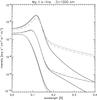 |
Fig. 6 Comparison between PRD and CRD profiles for D = 1000 km and T = 8000 K. Profiles with increasing intensity correspond to increasing gas pressures p = 0.001,0.1, and 0.5 dyne cm-2. Black profiles correspond to PRD and gray ones to CRD having enhanced wings. For hydrogen, which determines the electron density, the PRD approach was used for Lyman α and Lyman β lines. The gray dash then shows the effect of using CRD for both hydrogen and Mg ii. |
4.4. Models with PCTR and Mg II ionization
At temperatures lower than 104 K, the magnesium is practically in the state of Mg ii, see Morozhenko (1984) and references therein. We thus neglect a small fraction of Mg i, which was estimated to be 0.1−1% of Mg ii under prominence conditions. However, increasing the temperature within the PCTR leads to an increase of Mg iii ion population, as we show in Fig. 7. Here, Mg = Mg ii + Mg iii, if we neglect Mg i. At temperatures between 1.5 − 2 × 10⁴ K, Mg iii starts to dominate over Mg ii. For Mg iii, we consider only the ground state, and thus we cannot estimate the brightness of any lines belonging to Mg iii here. However, observing such lines could provide us with reliable diagnostics of the PCTR temperature structure. We will consider this problem in the next study when fully 2D fine-structure thread models of Gunár et al. (2008) will be used to synthesize the lines of magnesium and calcium at various ionization stages. Here, we only show an example of the Mg ii k line profiles that emerge from 1D slabs with the PCTR specified in Table 1. In Fig. 8, we see that the line core of the Mg ii k line is enhanced in the presence of the PCTR, as compared to the isothermal model with the same temperature as the central temperature in the PCTR model. The intensity enhancement is more pronounced for lower γtr values, which correspond to a spatially more extended PCTR and a narrower cool core. Notice the linear scale, which better shows the intensity enhancement in the line core affected by the PCTR.
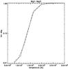 |
Fig. 7 Ionization degree Mg iii/Mg , as a function of the kinetic temperature for two PCTR models from Table 1. Full line for γ = 10 and dashed line for γ = 50. |
 |
Fig. 8 Mg ii k line profiles for two PCTR models from Table 1. The full thin line is for γtr = 10 and the dashed line for γtr = 50. The thick line corresponds to an isothermal model with T = 8000 K. |
5. Doppler brightening/dimming in Mg ii lines
Prominence spectral lines formed by the resonance scattering of the incident solar radiation are sensitive to the so-called Doppler-brightening or dimming effect, provided that the incident radiation is strongly varying within the wavelength range of a given spectral line. This was demonstrated theoretically for hydrogen lines by Heinzel & Rompolt (1987, see also references therein) and used by Gontikakis et al. (1997) to study the behavior of Lyman lines in eruptive prominences. The Doppler dimming was then studied also for helium lines, especially for HeII 304 Å (Labrosse et al. 2007; Labrosse & McGlinchey 2012). In the case of Mg ii resonance lines studied in this paper, one would also expect a pronounced effect, similar to the situation with hydrogen Lyman α. Our numerical code allows to account for the effects of macroscopic velocities on the radiation scattering by using a schematic approach as described in Heinzel & Rompolt (1987). The 1D prominence slab is illuminated on both sides symmetrically by the incident solar radiation, which is averaged over all incoming directions, and for each incident ray, we take into account the Doppler shift of this radiation due to the projection of the prominence velocity vector into the direction of a given ray. Then the 1D radiative transfer is simply solved subject to such velocity-dependent boundary conditions. A more sophisticated approach would be to account for the influence of all boundaries in 2D or even 3D.
For exploratory modeling in this paper, we use the same height above the surface H = 10 000 km as for all previous static models. In reality, the eruptive prominences can reach much larger altitudes and this affects the dilution factor for the incident radiation and also enhances the anisotropy of the incident radiation field. We used the range of velocities from 0 to 300 km s-1, and our results are shown in Fig. 9. For vt = 5 km s-1, we see that the k-line is brightened as the prominence moves radially upward or downward with velocities up to about 30 km s-1, with a maximum increase of more than 10%. This Doppler brightening is due to the strongly reversed profile of the incident chromospheric radiation. For higher velocities, the incident radiation is already dominated by the line wings, and we detect the Doppler dimming, which is quite important at high velocities. For larger microturbulent velocities, we see only the Doppler dimming because the strongly broadened line absorption profile acts in the wings of the incident profiles already for small velocities.
 |
Fig. 9 Examples of the Doppler dimming effect on the Mg ii k line. Shown is the dimming factor versus radial velocity, where the dimming factor is defined as the ratio of the line integrated intensity at a given velocity to the intensity at zero velocity. The plots correspond to models with D = 1000 km, T = 8000 K, p = 0.1 dyne cm-2, and two different turbulent velocities of 5 km s-1 (full line) and 20 km s-1 (dashed line). |
As stated above, we have averaged the incident radiation over all directions but also took the average for two wavelengths equally spaced from the line center (for details see Heinzel & Rompolt 1987). This means that our incident radiation has a symmetrical line profile with respect to the line center. However, due to the Doppler shift, the prominence is in reality illuminated by an asymmetrical radiation. In the case of CRD, this does not play any role since the photons are completely redistributed after the first scattering in optically thick slabs. However, the asymmetrical illumination is scattered quasi-coherently in the wings in the case of PRD, and this may lead to an asymmetry of the emergent line profile. This effect was demonstrated for hydrogen Lyman lines by Gontikakis et al. (1997).
6. Radiative losses in Mg ii lines
Radiative-equilibrium (RE) temperatures at slab center and at its surface (in parentheses).
It is well known that the radiative losses are dominated by hydrogen, Ca ii and Mg ii lines under the solar chromospheric conditions. In this section we always mean the net radiative losses, which include also the radiative heating. According to Vernazza et al. (1981, see their Table 29), the line losses integrated through the whole chromosphere are 30 × 105 erg s-1 cm-2 for Ca ii lines (two resonance lines plus the infrared triplet) and 9 × 10⁵ erg s-1 cm-2 for resonance lines of Mg ii. This was computed using the PRD approach for both Ca ii and Mg ii resonance lines. For a more recent modeling see Carlsson & Leenaarts (2012). Therefore, Mg ii contributes by less than 25% to these losses and, therefore, we have neglected them in our recent radiation-equilibrium (RE) models of 1D prominence slabs (Heinzel & Anzer 2012). These RE models, which include Ca ii losses, exhibit a substantial decrease of the radiation-equilibrium temperatures in 1D slabs as compared to the pure hydrogen case previously studied by Gouttebroze (2007). Having established the Mg ii line-formation behavior in prominences, we have solved the same RE relaxation problem, which now includes the hydrogen, Ca ii, and Mg ii radiative losses in the energy equation. The Ca ii H and K, Mg ii h and k, and hydrogen Lyman α and β lines are all computed with PRD. In Table 3, we present models for three gas pressures and prominence thicknesses. For all nine models, we start from a uniform temperature of 10 000 K, and let the prominence slab relax to RE. Resulting RE temperatures at the slab center and surface are summarized in Table 3, which is similar to that in Heinzel & Anzer (2012). We also compare our new results with the pure hydrogen case and hydrogen-calcium mixture. In the latter case, we have updated our previous Ca ii modeling, and thus, small differences appear in the present table as compared to that in Heinzel & Anzer (2012).
Inspection of Table 3 shows that the RE temperatures are generally lower than before, which is the natural consequence of adding Mg ii losses. The effect is rather marginal for the highest gas pressure 0.5 dyne cm-2 but increases substantially toward low pressures. For p = 0.01 dyne cm-2, the effect of Mg ii lines is quite large and much more important than that of Ca ii found earlier in Heinzel & Anzer (2012). This behavior can be explained by the much larger opacity of Mg ii lines in prominence slabs as compared to Ca ii lines. The opacity is so large at high pressures that the Mg ii radiative losses are significantly reduced. On the other hand, they become dominant over those of Ca ii at low pressures.
It is very interesting to observe that the RE temperatures for narrow slabs of 200 km are between 6000 and 8000 K for pressures between 0.01−0.1 dyne cm-2, which is quite compatible with most of observations. Even larger structures up to 1000 km show a similar behavior. If we could identify such narrow low-pressure slabs with the prominence fine structures (see e.g. Jejčič et al. 2013), our RE models would represent the energy-balance solution without any extra heating apart from the radiative heating by the solar illumination which is consistently accounted for in the form of gains in our net losses. For the model with the largest optical thickness (D = 5000 km, p = 0.5 dyne cm-2), the RE temperature in the slab center is somewhat larger than that computed without Mg ii. We have performed several numerical tests, but these higher temperatures remained there. One could thus speculate that this behavior is due to the very large optical depth, which becomes comparable to the thermalization depth, and thus, the Mg ii lines do not cool the plasma but slightly heat it at central parts of the slab. Detailed inspection of radiative losses at central parts being in RE indeed shows that the Mg ii losses are negative (meaning heating), while Ca ii ones are still positive, but about double in value than for the case without magnesium. This means that the RE temperature must be higher as compared to the case where the Mg ii losses were neglected. For smaller optical depths (all other models), this “heating” is not present, and there is a clear trend of stronger Mg ii radiative cooling when the optical thickness of the slab decreases with decreasing D and/or p. There is also a slight dependence on temperature.
7. Discussion and conclusions
In this study, we have calculated the profiles of the Mg ii h and k lines in solar prominences. All our models are based upon 1D isobaric vertical slab configurations. We selected a set of models with different values for the geometrical thickness and the gas pressure. We considered different types of temperature models. The models either have a constant temperature, allow for the presence of a PCTR, or are in radiative equilibrium. The line profiles, which we have obtained, can then be used as a prototype of the diagnostic tool for the IRIS observations.
There are several interesting aspects of these profiles. Profiles without any central reversal occur only for the lowest gas pressure values. The central intensity depends mainly on the temperature considered, and for the higher gas pressures, the line reversal increases strongly with the temperature. The line width (FWHM) is influenced both by the gas pressure and the thickness of the slab. We also considered the effect, which the presence of a PCTR has on the lines. We found that an extended PCTR can reduce the amount of the central reversal considerably but can increase the line-center intensity well above the limit of the diluted incident radiation at the same time. This demonstrates the sensitivity of the line core to the temperature structure of the PCTR. Next, we have studied the Doppler brightening/dimming of these lines. For quiescent prominences, which have typical macroscopic velocities below say 20 km s-1, the effect is almost negligible but it can be very important in the case of eruptive prominences. In addition, we extended our previous study of the radiative equilibrium in prominences (Heinzel & Anzer 2012) by including an additional cooling term, which is due to the presence of the Mg ii lines. We found that the effect can be important only in the case of the lowest pressures. For all others with more realistic gas pressure values, the resulting temperature changes are not so large.
Finally, we want to point out the importance of large opacities found for Mg ii lines. In this case, one should be able to see individual fine structures in high-resolution images taken by IRIS, in contrast to high-resolution Hα images where a substantial LOS integration is supposed to play a role because of the low opacities. For example, if two fine-structure threads are moving in different directions, the crossing point may give the impression that we see a moving bright blob. In Mg ii images, however, such a bright moving blob should be clearly distinguished from the crossing of two threads because of the large optical thickness of the Mg ii lines.
The exploratory models described in this paper are all based on very simple 1D slab configurations, while the quiescent prominences contain a large amount of fine structures. At present, we cannot judge what effect these fine structures will have on the results. Therefore, we plan to continue our analysis by using the 2D multithread models, which have been developed by Gunár et al. (2008). This will allow a more realistic modeling required for the detailed analysis of high-resolution IRIS data. Note that such modeling has been proven to be very successful in the case of hydrogen Lyman lines, as observed by SOHO/SUMER (Gunár 2013).
Acknowledgments
P.H. and U.A. thank the MPA and the Ondřejov Observatory, respectively, for support and hospitality during their mutual visits. This work was partially supported by the grants 209/12/0906, 209/11/2463 and 205/09/1705 of the Grant Agency of the Czech Republic. It was also supported by project RVO 67985815. We thank Gene Avrett and Han Uitenbroek for providing us with the atomic parameters and transition rates for Mg ii-Mg iii model atom. The authors thank Alan Title (LMSAL) for his support and for providing Fig. 1, and the referee T. M. D. Pereira for his comments and suggestions.
References
- Adams, T. F., Hummer, D. G., & Rybicki, G. B. 1971, J. Quant. Spectrosc. Radiat. Transfer, 11, 1365 [Google Scholar]
- Anzer, U., & Heinzel, P. 1999, A&A, 349, 974 [NASA ADS] [Google Scholar]
- Artzner, G., Vial, J. C., Lemaire, P., Gouttebroze, P., & Leibacher, J. 1978, ApJ, 224, L83 [NASA ADS] [CrossRef] [Google Scholar]
- Avrett, E., Landi, E., & McKillop, S. 2013, ApJ, 779, 155 [NASA ADS] [CrossRef] [Google Scholar]
- Berger, T. E., Shine, R. A., Slater, T. D., et al. 2008, ApJ, 676, 89 [Google Scholar]
- Bommier, V., Leroy, J. L., & Sahal-Bréchot, S. 1986, A&A, 156, 90 [NASA ADS] [Google Scholar]
- Bonnet, R. M., Blamont, J. E., & Gildwarg, P. 1967, ApJ, 148, L115 [NASA ADS] [CrossRef] [Google Scholar]
- Carlsson, M., & Leenaarts, J. 2012, A&A, 539, 39 [Google Scholar]
- De Pontieu, B., Title, A. M., Lemen, J. R. et al. 2014, Sol. Phys., DOI: 10.1007/s11207-014-0485-y [Google Scholar]
- Doschek, G. A., & Feldman, U. 1977, ApJS, 35, 471 [NASA ADS] [CrossRef] [Google Scholar]
- Dumont, S. 1967a, Ann. Astrophys. 30, 421 [Google Scholar]
- Dumont, S. 1967b, Ann. Astrophys. 30, 861 [Google Scholar]
- Engvold, O., Hirayama, T., Leroy, J.-L., Priest, E. R., & Tandberg-Hanssen, E. 1990, in Dynamics of Quiescent Prominences, eds. V. Ruždjak & E. Tandberg-Hanssen (Berlin: Springer-Verlag), Proc. IAU Coll. 117, Lect. Notes Phys., 363, 294 [Google Scholar]
- Fredga, K. 1969, Solar Phys., 9, 358 [NASA ADS] [CrossRef] [Google Scholar]
- Gontikakis, C., Vial, J. C., & Gouttebroze, P. 1997, A&A, 325, 803 [NASA ADS] [Google Scholar]
- Gouttebroze, P. 2007, A&A, 465, 1041 [NASA ADS] [CrossRef] [EDP Sciences] [Google Scholar]
- Gouttebroze, P., & Heinzel, P. 2002, A&A, 385, 273 [NASA ADS] [CrossRef] [EDP Sciences] [Google Scholar]
- Gouttebroze, P., Heinzel, P., & Vial, J.-C. 1993, A&AS, 99, 513 (GHV) [NASA ADS] [Google Scholar]
- Gunár, S. 2013, in Nature of Prominences and their Role in Space Weather, eds. B. Schmieder, J.-M. Malherbe, & S. T. Wu, Proc. IAUS300 (Cambridge Univ. Press), 59 [Google Scholar]
- Gunár, S., Heinzel, P., Anzer, U., & Schmieder, B. 2008, A&A, 490, 307 [NASA ADS] [CrossRef] [EDP Sciences] [Google Scholar]
- Heinzel, P. 1983, Bull. Astron. Inst. Czechoslov., 34, 1 [NASA ADS] [Google Scholar]
- Heinzel, P. 1995, A&A, 299, 563 [NASA ADS] [Google Scholar]
- Heinzel, P., & Anzer, U. 2012, A&A, 539, 49 [Google Scholar]
- Heinzel, P., & Hubeny, I. 1982, J. Quant. Spectrosc. Radiat. Transfer, 27, 1 [NASA ADS] [CrossRef] [Google Scholar]
- Heinzel, P., & Hubeny, I. 1984, J. Quant. Spectrosc. Radiat. Transfer, 30, 77 [NASA ADS] [CrossRef] [Google Scholar]
- Heinzel, P., & Rompolt, B. 1987, Sol. Phys., 110, 171 [NASA ADS] [CrossRef] [Google Scholar]
- Heinzel, P., Gouttebroze, P., & Vial, J.-C. 1987, A&A, 183, 351 [NASA ADS] [Google Scholar]
- Jejčič, S., Heinzel, P., Zapiór, M., et al. 2014, Sol. Phys., DOI: 10.1007/s11207-014-0482-1 [Google Scholar]
- Labrosse, N., & McGlinchey, K. 2012, A&A, 537, 100 [Google Scholar]
- Labrosse, N., Gouttebroze, P., & Vial, J. C. 2007, A&A, 463, 1171 [NASA ADS] [CrossRef] [EDP Sciences] [Google Scholar]
- Labrosse, N., Heinzel, P., Vial, J. C., et al. 2010, Space Sci. Rev., 151, 243 [Google Scholar]
- Leenaarts, J., Pereira, T. M. D., Carlsson, M., Uitenbroek, H., & De Pontieu, B. 2013a, A&A, 772, 89 [Google Scholar]
- Leenaarts, J., Pereira, T. M. D., Carlsson, M., Uitenbroek, H., & De Pontieu, B. 2013b, A&A, 772, 90 [Google Scholar]
- Lemaire, P., & Skumanich, A. 1973, A&A, 22, 61 [NASA ADS] [Google Scholar]
- Lemaire, P., Gouttebroze, P., Vial, J. C., & Artzner, G. E. 1981, A&A, 103, 160 [NASA ADS] [Google Scholar]
- Lemaire, P., Choucq-Bruston, M., & Vial, J. C. 1984, Sol. Phys., 90, 63 [NASA ADS] [CrossRef] [Google Scholar]
- Lites, B. W., & Skumanich, A. 1982, ApJS, 49, 293 [NASA ADS] [CrossRef] [Google Scholar]
- Milkey, R. W., & Mihalas, D. 1974, ApJ, 192, 769 [NASA ADS] [CrossRef] [Google Scholar]
- Mihalas, D., Auer, L. H., & Mihalas, B. R. 1978, ApJ, 220, 1001 [NASA ADS] [CrossRef] [Google Scholar]
- Morozhenko, N. N. 1984, Spectrophotometric study of quiescent solar prominences (Kiev: Naukova Dumka) [Google Scholar]
- Paletou, F. 1995, A&A, 302, 587 [NASA ADS] [Google Scholar]
- Paletou, F., Vial, J.-C., & Auer, L. H. 1993, A&A, 274, 571 [NASA ADS] [Google Scholar]
- Pereira, T. M. D., Leenaarts, J., De Pontieu, B., Carlsson, M., & Uitenbroek, H. 2013, A&A, 778, 143 [Google Scholar]
- Rybicki, G. B., & Hummer, D. G. 1991, A&A, 245, 171 [NASA ADS] [Google Scholar]
- Sigut, T. A. A., & Pradhan, A. K. 1995, J. Phys. B, 28, 4879 [Google Scholar]
- Skumanich, A. 1967, AJ, 72, 828 [NASA ADS] [CrossRef] [Google Scholar]
- Staath, E., & Lemaire, P. 1995, A&A, 295, 517 [NASA ADS] [Google Scholar]
- Tandberg-Hanssen, E. 1995, The Nature of Solar Prominences (Dordrecht: Kluwer) [Google Scholar]
- Uitenbroek, H. 1997, Sol. Phys., 172, 109 [NASA ADS] [CrossRef] [Google Scholar]
- Vernazza, J. E., Avrett, E. H., & Loeser, R. 1981, ApJS, 45, 635 [NASA ADS] [CrossRef] [Google Scholar]
- Vial, J.-C. 1982a, ApJ, 253,330 [NASA ADS] [CrossRef] [Google Scholar]
- Vial, J.-C. 1982b, ApJ, 254, 780 [NASA ADS] [CrossRef] [Google Scholar]
- Vial, J. C., Gouttebroze, P., Artzner, G., Lemaire, P. 1979, Sol. Phys. 61, 39 [NASA ADS] [CrossRef] [Google Scholar]
All Tables
Theoretical Mg ii h and k line parameters for 1D isothermal-isobaric prominence slabs.
Radiative-equilibrium (RE) temperatures at slab center and at its surface (in parentheses).
All Figures
|
Fig. 1 Uncalibrated stigmatic spectra of the Mg ii k (2795.53 Å) and h (2802.71 Å) lines detected by IRIS at 16:48:59 on July 18, 2013. The upper part of the figure, where the profiles are narrow, corresponds to a prominence seen above the South Pole limb. The lower part of the figure, where profiles are wide and reversed, corresponds to the chromosphere close to (and just above) the limb. The spectrum starts (left) at 2792.78 Å and ends (right) at 2805.34 Å. The spatial extension is 85 arcsec (Courtesy A. Title − LMSAL). |
| In the text | |
|
Fig. 2 Mg ii k line profiles of the normally emergent radiation from slabs with D = 200 km. The three sets of curves, increasing in their intensity, correspond to three gas pressures p = 0.01, 0.1, and 0.5 dyne cm-2. The gray scale corresponds to three temperatures: T = 6000 K (black), 8000 K (dark gray), and 10 000 K (light gray). Only one half of the symmetrical profiles is displayed. |
| In the text | |
 |
Fig. 3 Same as in Fig. 2, but for D = 1000 km. |
| In the text | |
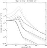 |
Fig. 4 Same as in Fig. 2, but for D = 5000 km. Note different intensity scale in this figure. |
| In the text | |
|
Fig. 5 Mg ii k line profiles of the normally emergent radiation from the slab with D = 1000 km and T = 8000 K. The two sets of curves correspond to values of the gas pressure p = 0.01 and 0.1 dyne cm-2. For each pressure, three curves show an increasing line broadening for the three values of the microturbulent velocity: 0 km s-1 (black), 3 km s-1 (dark gray), and 8 km s-1 (light gray). |
| In the text | |
|
Fig. 6 Comparison between PRD and CRD profiles for D = 1000 km and T = 8000 K. Profiles with increasing intensity correspond to increasing gas pressures p = 0.001,0.1, and 0.5 dyne cm-2. Black profiles correspond to PRD and gray ones to CRD having enhanced wings. For hydrogen, which determines the electron density, the PRD approach was used for Lyman α and Lyman β lines. The gray dash then shows the effect of using CRD for both hydrogen and Mg ii. |
| In the text | |
|
Fig. 7 Ionization degree Mg iii/Mg , as a function of the kinetic temperature for two PCTR models from Table 1. Full line for γ = 10 and dashed line for γ = 50. |
| In the text | |
|
Fig. 8 Mg ii k line profiles for two PCTR models from Table 1. The full thin line is for γtr = 10 and the dashed line for γtr = 50. The thick line corresponds to an isothermal model with T = 8000 K. |
| In the text | |
|
Fig. 9 Examples of the Doppler dimming effect on the Mg ii k line. Shown is the dimming factor versus radial velocity, where the dimming factor is defined as the ratio of the line integrated intensity at a given velocity to the intensity at zero velocity. The plots correspond to models with D = 1000 km, T = 8000 K, p = 0.1 dyne cm-2, and two different turbulent velocities of 5 km s-1 (full line) and 20 km s-1 (dashed line). |
| In the text | |
Current usage metrics show cumulative count of Article Views (full-text article views including HTML views, PDF and ePub downloads, according to the available data) and Abstracts Views on Vision4Press platform.
Data correspond to usage on the plateform after 2015. The current usage metrics is available 48-96 hours after online publication and is updated daily on week days.
Initial download of the metrics may take a while.