| Issue |
A&A
Volume 556, August 2013
|
|
|---|---|---|
| Article Number | A61 | |
| Number of page(s) | 12 | |
| Section | Astrophysical processes | |
| DOI | https://doi.org/10.1051/0004-6361/201321847 | |
| Published online | 26 July 2013 | |
Fragmentation of electric currents in the solar corona by plasma flows
1
Astronomical Institute,
AV ČR, Fričova 298,
25165
Ondřejov,
Czech Republic
e-mail:
This email address is being protected from spambots. You need JavaScript enabled to view it.
2
Max-Planck Institute for Solar System Research,
Katlenburg-Lindau, Max-Planck
Strasse 2, 37191
Katlenburg-Lindau,
Germany
Received:
6
May
2013
Accepted:
14
June
2013
Abstract
Aims. We consider a magnetic configuration consisting of an arcade structure and a detached plasmoid, resulting from a magnetic reconnection process, as is typically found in connection with solar flares. We study spontaneous current fragmentation caused by shear and vortex plasma flows.
Methods. An exact analytical transformation method was applied to calculate self-consistent solutions of the nonlinear stationary magnetohydrodynamic equations. The assumption of incompressible field-aligned flows implies that both the Alfvén Mach number and the mass density are constant on field lines. We first calculated nonlinear magnetohydrostatic equilibria with the help of the Liouville method, emulating the scenario of a solar eruptive flare configuration with plasmoids (magnetic ropes or current-carrying loops in 3D) and flare arcade. Then a Mach number profile was constructed that describes the upflow along the open magnetic field lines and implements a vortex flow inside the plasmoid. This Mach number profile was used to map the magnetohydrostatic equilibrium to the stationary one.
Results. We find that current fragmentation takes place at different locations within our configuration. Steep gradients of the Alfvén Mach number are required, implying the strong influence of shear flows on current amplification and filamentation of the magnetohydrostatic current sheets. Crescent- or ring-like structures appear along the outer separatrix, butterfly structures between the upper and lower plasmoids, and strong current peaks close the lower boundary (photosphere). Furthermore, impressing an intrinsic small-scale structure on the upper plasmoid results in strong fragmentation of the plasmoid. Hence fragmentation of current sheets and plasmoids is an inherent property of magnetohydrodynamic theory.
Conclusions. Transformations from magnetohydrostatic into magnetohydrodynamic steady-states deliver fine-structures needed for plasma heating and acceleration of particles and bulk plasma flows in dissipative events that are typically connected to magnetic reconnection processes in flares and coronal mass ejections.
Key words: magnetohydrodynamics (MHD) / Sun: flares / Sun: corona / methods: analytical
© ESO, 2013
1. Introduction
In the standard flare scenario (e.g., Magara et al. 1996) the energy release of the primary flare (primary magnetic reconnection) takes place in the current sheet below a rising magnetic rope. Here, the plasmoids (the secondary magnetic ropes in 3D), which are a natural outcome of the reconnection process, are formed and ejected. The ejection of plasmoids can be traced observationally via soft X-ray and radio waves, which map the magnetic-field reconnection (Ohyama & Shibata 1998; Kliem et al. 2000; Karlický et al. 2002; Karlický 2004). With increasing spatial resolution of the solar photosphere and chromosphere, flares, jets, and plasmoids on different scales are observed (e.g., Cargill 2013; Cirtain et al. 2013). This means that the solar atmosphere is highly structured, and magnetic reconnection processes are ubiquitous. As such, the current sheets initiating reconnection processes cannot be smooth but must contain some internal fragmented structure. Consequently, magnetic reconnection itself must be fractal. As an efficient mechanism to cascade down to smaller scales, instabilities have proven to be an ideal trigger.
Many nonlinear, time-dependent magnetohydrodynamic (MHD) simulations focus on linear and nonlinear instabilities, which are initiated via arbitrarily prescribed small perturbations of an initially smooth, static equilibrium. These instabilities typically result in reconnection, and in the following in fragmentation of the magnetic field and hence the current density (e.g., Bárta et al. 2010; Karlický & Bárta 2011; Bárta et al. 2011), forming chains of plasmoids (Loureiro et al. 2007; Uzdensky et al. 2010), coalescence and further fragmentation of plasmoids (Pegoraro et al. 2010; Karlický & Bárta 2011), and plasmoids on progressively smaller scales (Shibata & Tanuma 2001).
The process of cascading can also be initiated by stochastic velocity fluctuations, generating small-scale structures of the large-scale magnetic field (Lazarian & Vishniac 1999; Kowal et al. 2009; Eyink 2011). This turbulent approach, however, originates from external perturbations impressed on initial background (magnetic and velocity) fields, requiring the prescription of initial noise, e.g., in the form of power-law spectra of perturbations. On the other hand, the turbulent reconnection can result from a successive coalescence and fragmentation of plasmoids, their fast heating, and an increase of the plasma beta parameter at some locations, where the flow instabilities become important as well (Karlický et al. 2012).
In contrast to studies using instabilities or turbulence as the initial trigger for fragmentation, the MHD theory itself inherently provides the cradles for fractal structures, because the MHD is scale-free and therefore applies to large as well as to small scales (Shibata 2012a,b). In their studies of the Earth’s magnetotail using a quasi-static adiabatic MHD approach, Wiegelmann & Schindler (1995) previously noticed the fragmentation of a thin current sheet. In their investigations, they found the formation of double-structures of the current density when using nonsimilarity solutions of the quasi-static equations. Similarly, the numerical investigations of Becker et al. (2001) revealed the formation of thin current sheets from a sequence of static equilibria. Thus, instead of using perturbations of a smooth, static equilibrium, one might start directly from already structured, fragmented MHD equilibrium states. For this, one needs to construct a selfconsistent analytical description of the time-independent, nonlinear dynamics (see, e.g., Nickeler & Fahr 2001; Nickeler et al. 2006; Nickeler & Wiegelmann 2010, 2012).
Separatrices form during magnetic reconnection processes, which originate in so-called X-points. These X-points can separate regions of closed and open field lines. The open field-line regions can be regarded as field lines along which, e.g., the solar wind can flow into the interplanetary space, while the closed regions correspond to, e.g., magnetic arcades or flux ropes (plasmoids) from which plasma cannot leave. To stabilize such a configuration, in which strong flows occur outside and (almost) no flows inside, shear currents have to keep the system in equilibrium. Hence the physical problem can be approximately described with the static approach in regions of closed field lines, while in regions with open field lines the problem is in steady-state (see, e.g., Nickeler et al. 2006; Nickeler & Wiegelmann 2010, 2012).
Nickeler & Wiegelmann (2010) considered that the Alfvén Mach number, MA, determining the strength of the flow and therefore the plasma velocity, vanishes within the plasmoid, so that the structure is basically magneto-hydrostatic (MHS). However, not every closed field-line region must necessarily be of MHS nature. Instead, plasmoids might contain vortices, because slight asymmetries during the ejection event could result in a nonzero angular momentum transfer. Hence the flow inside plasmoids can be sheared. Shear flows were found to produce current filamentation not only in solar or magnetospheric environments, but also in space and astrophysical plasmas, e.g., in astrophysical jets, where shear flows also induce the filamentation of currents (Wiechen et al. 1998; Konz et al. 2000).
In this paper, we investigate the role of shear flows within a configuration containing a magnetic dome and detached plasmoids, resembling a typical solar-flare configuration after a first reconnection process. In our investigations, we used a selfconsistent analytical description of the time-independent, nonlinear dynamics. The paper is structured as follows: in Sect. 2 we introduce the basic equations and the transformation method, while the results are described in Sect. 3. The assumptions are discussed in Sect. 4, and the conclusions are given in Sect. 5.
2. Basic equations
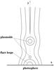 |
Fig. 1 Sketch of a magnetic configuration of a solar flare with plasmoids formed via magnetic reconnection processes. |
We assumed a magnetic configuration of a solar flare with a plasmoid formed via some first magnetic reconnection event (see Fig. 1). The plasmoid is enclosed by two X-points, while the plasmoid itself hosts a magnetic O-point in its center. The equilibrium of such a system can be formulated using the steady/static approach. This is, however, only strictly valid if the plasmoid has no or only marginal motion in y direction. The dynamics of plasmoids depends on the reconnection rate at the X-points below and above the plasmoid, and plasmoids “in rest” (see, e.g., Bárta et al. 2008a,b) and stable (i.e. without further coalescence, see, e.g., Knoll & Chacón 2006) have been found by numerical simulations, justifying our assumption.
The choice of a certain equilibrium defines an arbitrary, but fixed length-scale. This does
not allow one to make inferences on the properties of the plasmoid on (much) smaller scales,
on which, e.g., stationary shear flows related to vortex sheets might exist. Such shear
flows would generate additional forces on the former MHS states, which can only be
compensated for by changes in Lorentz forces and pressure gradients. To maintain the force
balance self-consistently, we applied the transformation method developed by Gebhardt & Kiessling (1992) and
advanced/progressed by Petrie & Neukirch
(1999) and Nickeler et al. (2006). In the
past decades many attempts have been made to find exact and analytical solutions of
nonlinear steady-state (=stationary) MHD equations (e.g., Tsinganos 1981; Contopoulos 1996; Goedbloed & Lifschitz 1997; Nickeler & Fahr 2005, 2006). However, the transformation is the only systematic method that physically and
mathematically relates steady-state MHD flows to MHS states. For such a transformation to
work, it is reasonable to request that in the stationary state the velocity field and the
magnetic field are parallel (field-aligned flows). This guarantees that the electric field
vanishes, according to the ideal Ohm’s law
 (1)We note that other
transformations between steady MHD states exist, which lead to configurations in which the
velocity field and the magnetic field are not necessarily parallel (Bogoyavlenskij 2000, 2001, 2002). However, only in the case of incompressible
field-aligned flows one can always reduce the steady-state MHD equations to the MHS
equations. Another advantage of the transformation method is that it is independent of the
dimensions, i.e., it can be performed in 1, 2, and 3D.
(1)We note that other
transformations between steady MHD states exist, which lead to configurations in which the
velocity field and the magnetic field are not necessarily parallel (Bogoyavlenskij 2000, 2001, 2002). However, only in the case of incompressible
field-aligned flows one can always reduce the steady-state MHD equations to the MHS
equations. Another advantage of the transformation method is that it is independent of the
dimensions, i.e., it can be performed in 1, 2, and 3D.
2.1. Transformation from MHS states to stationary MHD configurations
In the following we restrict the analysis to sub-Alfvénic flows to emphasize in
particular their relationship to MHS states. In addition, we use normalized parameters,
for which we introduce normalization constants  and
and  , where
 is the normalized Alfvén velocity. Let v be the plasma velocity normalized on
, ρ
the mass density normalized on
is the normalized Alfvén velocity. Let v be the plasma velocity normalized on
, ρ
the mass density normalized on  ,
j = ∇ × B the current density vector normalized on
,
j = ∇ × B the current density vector normalized on
 with
with  as the characteristic length scale, and p the scalar plasma pressure
normalized on
as the characteristic length scale, and p the scalar plasma pressure
normalized on  .
With these definitions, we can write the set of equations of stationary, field-aligned
incompressible MHD, consisting of the mass continuity equation, the Euler equation, the
definition for field-aligned flow and Alfvén Mach number, the incompressibility condition,
and the solenoidal condition for the magnetic field, in the form
.
With these definitions, we can write the set of equations of stationary, field-aligned
incompressible MHD, consisting of the mass continuity equation, the Euler equation, the
definition for field-aligned flow and Alfvén Mach number, the incompressibility condition,
and the solenoidal condition for the magnetic field, in the form  This
set of equations can always be reduced to the set of static equations using the
transformation equations (for details see Nickeler
& Wiegelmann 2010, 2012) of the
form
This
set of equations can always be reduced to the set of static equations using the
transformation equations (for details see Nickeler
& Wiegelmann 2010, 2012) of the
form  where
the subscript S refers to the original MHS fields. Here it is a necessary
condition that the Alfvén Mach number MA and the density
ρ are constant along fieldlines, i.e.,
where
the subscript S refers to the original MHS fields. Here it is a necessary
condition that the Alfvén Mach number MA and the density
ρ are constant along fieldlines, i.e.,  An
important property of this type of transformation is the fact that every transformed
magnetic field strength | B | is stronger than the original static magnetic
field strength | BS | (as long as
MA ≠ 0). Moreover, as j is directly proportional
to the term ∇MA, which can have an arbitrarily (but not
infinite) high value, basically every infinitesimale scale
1/∇ = l > 0 can be chosen.
Therefore, we can produce a current that is higher than any current threshold to excite
anomalous resistivity, such that current-driven instabilities and hence magnetic
reconnection can be induced. This generated current can be even more amplified when the
Alfvén Mach number approaches the limit MA ≲ 1. We stress that
the transformation method provides a nonlinear self-consistent solution of the stationary
MHD equations, and changing any of the physical variables produces a nonlinear feed-back
of all other variables. Variations of MA should not be
misunderstood as an explicit time-dependent change or sequence of the underlying MHS
equilibrium, like in the quasi-static sequences of Wiegelmann & Schindler (1995) or Becker
et al. (2001). Instead, the transformation has to be interpreted as a nonlinear
variation or displacement of the former initial MHS equilibrium. That is, in affinity to
variational calculus, the steady-states are “located” in the proximity of MHS states.
An
important property of this type of transformation is the fact that every transformed
magnetic field strength | B | is stronger than the original static magnetic
field strength | BS | (as long as
MA ≠ 0). Moreover, as j is directly proportional
to the term ∇MA, which can have an arbitrarily (but not
infinite) high value, basically every infinitesimale scale
1/∇ = l > 0 can be chosen.
Therefore, we can produce a current that is higher than any current threshold to excite
anomalous resistivity, such that current-driven instabilities and hence magnetic
reconnection can be induced. This generated current can be even more amplified when the
Alfvén Mach number approaches the limit MA ≲ 1. We stress that
the transformation method provides a nonlinear self-consistent solution of the stationary
MHD equations, and changing any of the physical variables produces a nonlinear feed-back
of all other variables. Variations of MA should not be
misunderstood as an explicit time-dependent change or sequence of the underlying MHS
equilibrium, like in the quasi-static sequences of Wiegelmann & Schindler (1995) or Becker
et al. (2001). Instead, the transformation has to be interpreted as a nonlinear
variation or displacement of the former initial MHS equilibrium. That is, in affinity to
variational calculus, the steady-states are “located” in the proximity of MHS states.
The set of transformation equations (Eqs. (7)–(11)) together with the conditions of Eqs. (12), (13) provide a “recipe” to construct field-aligned, incompressible flows along the MHS structures. In practice, we first need to calculate an MHS equilibrium. In the following we assumed that the equilibrium has some sort of symmetry (e.g. in z-direction), so that it can be reduced to a pure 2-dimensional (2D) problem1. In that case, the equilibrium value of the magnetic field has the form BS = ∇A(x,y) × ez.
Next, we need to determine a Mach number profile,
MA(A). This profile has to depend locally
only on the flux function, A, so that
BS·∇MA = 0, and hence the condition
Eq. (12) is automatically fulfilled. The
“new” magnetic field, i.e., the steady-state field, is then given by a new flux function
α, which is a function of A, such that 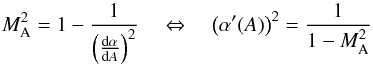 (14)and
B = ∇α × ez (see
Nickeler & Wiegelmann 2010). The prime
denotes the derivative with respect to A. Armed with this Mach number
profile and BS, the set of transformation equations (Eqs. (7) to (11)) can be evaluated.
(14)and
B = ∇α × ez (see
Nickeler & Wiegelmann 2010). The prime
denotes the derivative with respect to A. Armed with this Mach number
profile and BS, the set of transformation equations (Eqs. (7) to (11)) can be evaluated.
For the adopted 2D shape of the magnetic field the current-transformation equation (Eq.
(10)) takes the form 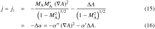 The
current fragmentation is strong where the magnetic field is strong, as the increase in
current and its spatial variation is mainly governed by
The
current fragmentation is strong where the magnetic field is strong, as the increase in
current and its spatial variation is mainly governed by
 but amplified
by (∇A)2.
but amplified
by (∇A)2.
One interesting and important property of this transformed current is the fact that it
can have a zero-crossing even for an initially monopolar MHS-current distribution. This
means that any suitable choice of a transformation can make
jz negative (positive), although the MHS
current is completely positive (negative). In particular, the zero-crossing of the current
requires that it has to vanish at some point, i.e.,
 . This delivers a condition for
the Mach number profile of the form
. This delivers a condition for
the Mach number profile of the form 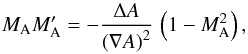 (17)with the restriction
(∇A)2 ≠ 0. As an important example of a monopolar
MHS-current we refer to Liouville’s equation given by
ΔA = exp(−2A) (see Eq. (20) below). Because ΔA is
always positive and (∇A)2 and
(17)with the restriction
(∇A)2 ≠ 0. As an important example of a monopolar
MHS-current we refer to Liouville’s equation given by
ΔA = exp(−2A) (see Eq. (20) below). Because ΔA is
always positive and (∇A)2 and
 are positive
as well, the left-hand side derivative of Eq. (17) must be negative, i.e.,
are positive
as well, the left-hand side derivative of Eq. (17) must be negative, i.e.,  . This condition can in
principle be fulfilled with any suitable Alfvén Mach number profile that is monotonically
decreasing with A (at least locally). This demonstrates the power of the
transformation method and shows that it can be used to generate strong current
fragmentation.
. This condition can in
principle be fulfilled with any suitable Alfvén Mach number profile that is monotonically
decreasing with A (at least locally). This demonstrates the power of the
transformation method and shows that it can be used to generate strong current
fragmentation.
The zero-crossing is a definite sign that fragmentation can take place, but in many cases
it is sufficient to have a strong gradient concerning MA
and/or a large (∇A)2. On the other hand, this means that in
the vicinity of a magnetic null point must be
extremely large to compensate the vanishing magnetic field strength. Nevertheless,
depending on the choice of the Mach number profile, current fragmentation can happen even
without a zero-crossing of the transformed current.
3. Results
3.1. Nonlinear static equilibria
As described in the previous section, the first step is to derive a reasonable initial MHS equilibrium, which is able to reproduce a field-line scenario with individual disconnected plasmoids, as drawn schematically in Fig. 1. For this, we used two well-known equilibrium configurations and combined them.
Starting from the static magnetic field in 2D,
BS = ∇A × ez,
and inserting it into the MHS equilibrium equation (Eq. (11)) delivers the well-known Grad-Shafranov-equation, often also called
Lüst-Schlüter-equation (see, e.g., Lüst & Schlüter
1957; Shafranov 1958) 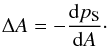 (18)Because
BS·∇A = 0 is valid, lines of constant
A are field lines. This implies that the current
j = −ΔA is constant along field lines, as is the
pressure pS, because they are functions of A,
and consequently the isocontours of the current have the same topological and geometrical
structure as those of the field lines.
(18)Because
BS·∇A = 0 is valid, lines of constant
A are field lines. This implies that the current
j = −ΔA is constant along field lines, as is the
pressure pS, because they are functions of A,
and consequently the isocontours of the current have the same topological and geometrical
structure as those of the field lines.
For the pressure function pS(A) we use
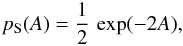 (19)as
derived in the frame of the Vlasov theory by, e.g., Bennett
(1934), Harris (1962), and Kan (1973). The same function is typically applied in
MHS or MHD configurations in which the pressure monotonically decreases in the direction
perpendicular to the current sheet. Examples are flare configurations, magnetotails, and
helmet streamers (see, e.g., Birn et al. 1975; Wiegelmann et al. 1998; Bárta et al. 2008a, 2010). With this
pressure function, the Grad-Shafranov-equation has the form
(19)as
derived in the frame of the Vlasov theory by, e.g., Bennett
(1934), Harris (1962), and Kan (1973). The same function is typically applied in
MHS or MHD configurations in which the pressure monotonically decreases in the direction
perpendicular to the current sheet. Examples are flare configurations, magnetotails, and
helmet streamers (see, e.g., Birn et al. 1975; Wiegelmann et al. 1998; Bárta et al. 2008a, 2010). With this
pressure function, the Grad-Shafranov-equation has the form 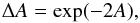 (20)also
known as Liouville’s equation (e.g., Bandle 1975).
(20)also
known as Liouville’s equation (e.g., Bandle 1975).
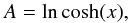
By defining u = x + iy,
ν= x − iy, and i2 = −1,
Liouville’s equation can be written as (see Bandle
1975; Birn et al. 1978) 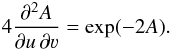 (21)The
general solution of Liouville’s equation, Eq. (21), is given by
(21)The
general solution of Liouville’s equation, Eq. (21), is given by 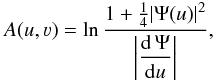 (22)implying
that every holomorphic function Ψ(u) gives us an exact solution of the
nonlinear Grad-Shafranov-equation, Eq. (20).
(22)implying
that every holomorphic function Ψ(u) gives us an exact solution of the
nonlinear Grad-Shafranov-equation, Eq. (20).
The classical ansatz is 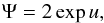 (23)leading to the
Harris-sheet equilibrium (Harris 1962)
(23)leading to the
Harris-sheet equilibrium (Harris 1962)
 (24)which represents a
bipolar magnetic field structure, i.e., a plasma or current sheet separating magnetic
fields with opposite orientations. This is a one-dimensional structure.
(24)which represents a
bipolar magnetic field structure, i.e., a plasma or current sheet separating magnetic
fields with opposite orientations. This is a one-dimensional structure.
A modified magnetic-field structure including a normal component penetrating the 2D
current sheet was calculated by Kan (1973) for the
case of the Earth’s magnetotail region. Such a configuration emulates the dipole structure
that extends into and influences the Earth’s magnetotail. In addition, with respect to
configurations within the solar corona, such a scenario ideally resembles, e.g., magnetic
dome structures. Kan (1973) chose the function
Ψ = 2exp(u + d/u),
which drops off for | u| → ∞. Here, d is a constant.
This choice is a slight perturbation of the original 1D Harris sheet toward a 2D
magnetic-field configuration, converging for large distances back again to the original
Harris-sheet equilibrium. The corresponding flux function is
![Mathematical equation: \begin{equation} A= \ln \displaystyle\frac{\cosh\left[ x\left(1+\frac{d}{r^{2}}\right)\right]} {\sqrt{\displaystyle\frac{(d^{2}-2d(x^{2}-y^{2})+r^{4})}{r^{4}}}} , \end{equation}](/articles/aa/full_html/2013/08/aa21847-13/aa21847-13-eq66.png) (25)where
(25)where
 .
The resulting field lines, computed for d = 0.5, are shown in the top
panel of Fig. 2, with the y-axis
pointing in magnetotail direction, and the Earth (in the original Kan picture) located at
the origin of the coordinate system. This scenario allows one to describe stretched,
tail-like structures, including a dipole-like configuration close to the Earth (i.e., for
low values of y).
.
The resulting field lines, computed for d = 0.5, are shown in the top
panel of Fig. 2, with the y-axis
pointing in magnetotail direction, and the Earth (in the original Kan picture) located at
the origin of the coordinate system. This scenario allows one to describe stretched,
tail-like structures, including a dipole-like configuration close to the Earth (i.e., for
low values of y).
To describe the field lines of periodic structures, we applied the approach of Schmid-Burgk (1967), who developed a formalism to solve
Liouville’s equation resulting in the so-called periodic, corrugated sheet-pinch. In this
scenario, the original Harris-sheet equilibrium is slightly modified to
 with δ as a constant, leading to the following flux function:
 (26)The field lines
evaluated for δ = 0.1 are shown in the middle panel of Fig. 2.
(26)The field lines
evaluated for δ = 0.1 are shown in the middle panel of Fig. 2.
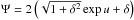
For our purposes, we used the approaches from both Kan and Schmid-Burgk, and combined
them, i.e., we applied the modification of the Harris-sheet found by Schmid-Burgk (1967) to the Kan equilibrium. This is necessary, because
we aim at achieving a representation in which the equilibrium has a strong
Bx-component close to the lower boundary
y = 0 and a periodic-sheet pinch for y → ∞. This means
that Ψ is now represented by 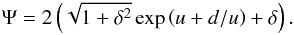 (27)With this function,
we finally obtain a flux function of the form
(27)With this function,
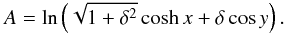
we finally obtain a flux function of the form ![Mathematical equation: \begin{equation} A = \ln\displaystyle\frac{\sqrt{1+\delta^{2}} \cosh\left[ x\left(1+\frac{d}{r^{2}}\right)\right] + \delta \cos\left[y\left(1-\frac{d}{r^{2}}\right)\right] } {\sqrt{\displaystyle\frac{(d^{2}-2d(x^{2}-y^{2})+r^{4})}{r^{4}}}} , \label{finalflux} \end{equation}](/articles/aa/full_html/2013/08/aa21847-13/aa21847-13-eq78.png) (28)whose contour plot has
field lines as depicted in the bottom panel of Fig. 2. In our representation the y-axis corresponds to the height
above the solar photosphere, and the photosphere itself is located at
y = 0. The symmetry axis of the post-flare magnetic field configuration
is given by x = 0. This flux function (Eq. (28)) is used in the following and serves as our initial MHS
equilibrium.
(28)whose contour plot has
field lines as depicted in the bottom panel of Fig. 2. In our representation the y-axis corresponds to the height
above the solar photosphere, and the photosphere itself is located at
y = 0. The symmetry axis of the post-flare magnetic field configuration
is given by x = 0. This flux function (Eq. (28)) is used in the following and serves as our initial MHS
equilibrium.
 |
Fig. 2 Field lines for the Kan magnetotail (top), the periodic sheet pinch or periodic Harris sheet (middle), and the combined one (bottom) that serves as our initial MHS equilibrium. |
3.2. Different transformation approaches
There exist three different approaches to model field aligned shear flows. These are the transformations via
-
magnetic field amplification defined by α′,
-
peaked plasma flows defined by MA, and
-
asymptotical 1D current structures defined by j.
Each approach requires the specification of either one of the finally transformed MHD values (such as the current or the magnetic field, the latter is even identical to the transformation itself), or the plasma flow of the stationary MHD configuration. In combination with the prescribed intrinsic MHS values, the corresponding transformation between these two states can be evaluated.
As we have shown, Eq. (14) describes two equivalent methods for a transformation, i.e., via the calculation of either the transformed magnetic field, specified by α′, or the plasma flow in the transformed configuration, given by MA. On the other hand, it is also reasonable to compute the Mach number profile via Eq. (15) by specifying the asymptotic behavior of the transformed current j. These three methods are basically equivalent, but each of them emphasizes a different physical aspect of the fragmentation problem, and consequently needs different constraints and boundary conditions. More specifically, each method is based on the prescription of one physical parameter that serves as control parameter.
3.2.1. Transformation via magnetic-field amplification defined by α′
The first mapping method has been described in detail by Nickeler et al. (2006). It is based on the prescription of the
magnetic field and is best applicable for potential fields that are asymptotical
homogeneous, i.e., their flux function is given by
A ≈ BS∞x for large
y. In that case, the transformation between the new, steady-state
flux function α and the old, stationary flux function
A is given by  This
transformation, which is based on the calculation of α′,
produces a series of k Harris-sheets with different strengths
ak/dk
and widths dk, offset by
Ak from the MHS state. The parameters
C, Ak,
ak, and
dk are not completely free. They have
to be chosen such that
|α′(A)| > 1 to
guarantee sub-Alfvénic flows and to satisfy the boundary conditions or constraints,
provided, e.g., by observations. The number of Harris-type current sheets
k depends on the number of separatrix lines originating in potential
X-points. This means that k is determined or fixed by the number of
“pauses”, i.e., boundary layers, within the chosen domain. The location of the pauses is
marked by Ak. Such transformations are
ideal for a proper modeling of tail configurations as they appear in the heliotail (or
astrotails in general, see Nickeler & Fahr
2001; Nickeler et al. 2006), which
require the maintenance of strong current sheets that form the boundary layer in the
vicinity of the seperatrix (heliopause/astropause) in between the outer solar/stellar
wind and the very local interstellar medium.
This
transformation, which is based on the calculation of α′,
produces a series of k Harris-sheets with different strengths
ak/dk
and widths dk, offset by
Ak from the MHS state. The parameters
C, Ak,
ak, and
dk are not completely free. They have
to be chosen such that
|α′(A)| > 1 to
guarantee sub-Alfvénic flows and to satisfy the boundary conditions or constraints,
provided, e.g., by observations. The number of Harris-type current sheets
k depends on the number of separatrix lines originating in potential
X-points. This means that k is determined or fixed by the number of
“pauses”, i.e., boundary layers, within the chosen domain. The location of the pauses is
marked by Ak. Such transformations are
ideal for a proper modeling of tail configurations as they appear in the heliotail (or
astrotails in general, see Nickeler & Fahr
2001; Nickeler et al. 2006), which
require the maintenance of strong current sheets that form the boundary layer in the
vicinity of the seperatrix (heliopause/astropause) in between the outer solar/stellar
wind and the very local interstellar medium.
3.2.2. Transformation via peaked plasma flows defined by MA
For the second possible transformation method a Mach number profile
MA(A) has to be specified. To obtain a
highly-structured current distribution, the Mach number profile needs to contain strong
gradients and must show strong spatial variation. This means that
MA cannot be given by a simple two-dimensional function,
but has to be constructed out of several pieces or branches, which need to be connected
by continuous transitions, meaning that each of these branches must be at least twice
continuously differentiable at the boundaries of the intervals so that no
discontinuities in the current density profile appear. Consequently, the function
MA must be composed of a set of functions
mk(A), which exist only
within some defined field-line interval and vanish outside. In addition, the functions
mk(A) must have a
compact support to guarantee that both  and
and
 ,
i.e., the Mach number and its constituents are bounded functions (sub-Alfvénic).
,
i.e., the Mach number and its constituents are bounded functions (sub-Alfvénic).
This goal can be achieved in different ways: (i) One may define piece-wise functions
that vanish at the boundary of some field-line interval; (ii) one may apply purely the
classical partition of unity; (iii) the partition of unity is used in combination with a
continuous sum, i.e., continuous distribution of flow tubes that can be written as an
integral. This means that we can define a general function for
MA of the form
 (31)which
consists of a sum over k individual peaked plasma flows, each defined
within discrete field-line intervals, and a continuous distribution
m(A) of plasma flow tubes.
(31)which
consists of a sum over k individual peaked plasma flows, each defined
within discrete field-line intervals, and a continuous distribution
m(A) of plasma flow tubes.
Such an approach with a pure continuous distribution m(A) ~ 1/cosh(A)2 has been used, e.g., by Nickeler & Wiegelmann (2010) to generate a single current-sheet along a magnetic separatrix. In contrast, we show in Sect. 3.3 an example in which piece-wise functions are defined.
3.2.3. Transformation via asymptotical 1D current structures defined by j: the inverse method
The third method to determine the transformation is based on the prescription of the transformed current, j, given by Eq. (15) (see also Nickeler et al. 2006). Typically, in magnetostatics the magnetic field is directly calculated from Ampère’s equation ΔA = −j, where the current distribution j is prescribed. In MHD, a prescription of the current distribution or the magnetic field is not possible. Here, the values have to be calculated self-consistently and simultaneously from the nonlinear MHD equations. But the transformation method enables us to define the current distribution in configurations that occur ubiquitously in space plasmas as an explicit function of the flux function A. If we can find a way to prescribe the current density j as a spatially, i.e., depending on A(x,y), strongly variable current distribution, we can generate self-consistently current fragmentations on small scales, emulating scenarios that in the literature are often approached via turbulence originating from external perturbations (Lazarian & Vishniac 1999; Kowal et al. 2009; Eyink 2011).
As was shown in Sect. 2.1, the current
distribution, resulting from the transformation, is given by 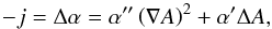 (32)with
j = jz(x,y).
The terms
α′′,α′, and
ΔA are pure functions of the flux function A. On the
other hand, the quadratic expression (∇A)2 is a scalar
function and generally a function of x and y, which,
in the case of 2D equilibria, cannot be expressed as an explicit function of
A only. Instead, Eq. (32) is an equation defining or rather determining
j(x,y) ≡ j(A,y)
from a given transformation α′, which seems to be the most
consequent and logical method. However, Eq. (32) cannot be regarded as just a pure ordinary differential equation for
α′. Therefore, calculating α′
from Eq. (32) for a given or prescribed
j, has in general no formal solution (see Appendix A). Based on this mathematical problem, it is
necessary to find a different approach.
(32)with
j = jz(x,y).
The terms
α′′,α′, and
ΔA are pure functions of the flux function A. On the
other hand, the quadratic expression (∇A)2 is a scalar
function and generally a function of x and y, which,
in the case of 2D equilibria, cannot be expressed as an explicit function of
A only. Instead, Eq. (32) is an equation defining or rather determining
j(x,y) ≡ j(A,y)
from a given transformation α′, which seems to be the most
consequent and logical method. However, Eq. (32) cannot be regarded as just a pure ordinary differential equation for
α′. Therefore, calculating α′
from Eq. (32) for a given or prescribed
j, has in general no formal solution (see Appendix A). Based on this mathematical problem, it is
necessary to find a different approach.
Magnetohydrostatic equilibria in space plasmas often have regions where the fields are extremely stretched. Such tail-like regions typically occur far away from bipolar or even multipolar field regions, as, e.g., in our case (bottom panel of Fig. 2) in the regions of high | x | values, or, in the case of the Kan equilibrium, also in the regions of high y values (top panel of Fig. 2), or in general for going to ∞ along or in the direction of the tail axis. The regions of stretched field lines can be approximated by a 1D configuration, which depends only weakly on a second coordinate. Examples are asymptotically 1D regions of exact and analytical tail equilibria or so-called weakly 2D or weakly 3D equilibria (see, e.g., Schindler 1972, 1979; Birn et al. 1977). The advantage of this asymptotically 1D approach is that the equilibrium problem can be treated as if it depended on only one coordinate. This coordinate is, at least locally, a unique function of the field-line label A, and vice versa, so that in a local coordinate system A can always be chosen as coordinate. Therefore, in these stretched field line regions, the problem can be solved. The solution found is, however, a general solution and not restricted to the pure 1D region, because every found solution for | α′| > 1 is an exact solution of the sub-Alfvénic steady-state problem (Eqs. (7)–(11)).
Assuming that
limx,y → ∞BS = BS∞,
we define
| BS∞| = BS∞(A).
The limes has to be smooth. Then we can introduce the asymptotical current via
∇ × (limx,y → ∞BS) = limx,y → ∞(∇ × BS) = limx,y → ∞jS,
with
limx,y → ∞|jS| = jS∞(A) = PS ′(A).
The last identification thereby again represents the Grad-Shafranov-equation (Eq. (18)). With these relations, Eq. (32) can be written as  (33)This
pure one-dimensional differential relation is now a linear ordinary differential
equation of first order for α′(A), which
can be solved: We divide both sides of Eq. (33) by
(33)This
pure one-dimensional differential relation is now a linear ordinary differential
equation of first order for α′(A), which
can be solved: We divide both sides of Eq. (33) by  and multiply with
the integrating factor
and multiply with
the integrating factor 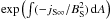 . This
leads to a complete differential that can be integrated, resulting in the following
general solution
. This
leads to a complete differential that can be integrated, resulting in the following
general solution 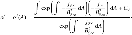 (34)Thus
for reasonable prescribed stationary asymptotic current densities
j∞(A), the general solution of the
transformation α′ can be computed from the asymptotic MHS
functions for the current density jS∞(A)
and the magnetic field BS∞(A). The
parameter C0 is an integration constant, defining an offset
and a boundary condition for α′, hence
MA.
(34)Thus
for reasonable prescribed stationary asymptotic current densities
j∞(A), the general solution of the
transformation α′ can be computed from the asymptotic MHS
functions for the current density jS∞(A)
and the magnetic field BS∞(A). The
parameter C0 is an integration constant, defining an offset
and a boundary condition for α′, hence
MA.
To find suitable prescriptions for j∞(A) that guarantee α′2 > 1 also in the two-dimensional regions is a difficult practical task. However, with this approach it is basically possible to generate current fragmentation scenarios based purely on the self-consistent solution of the MHD equations. Hence, the transformation method provides a self-consistent tool in which current fragmentation is a basic property of the nonlinear MHD theory, because j∞ is basically not subject to any limitations.
3.3. Example for shear-flow-induced current fragmentation
The aim of our analysis is to study the process of current fragmentation that takes place in the vicinity and within an ejected plasmoid that was formed via magnetic reconnection in a typical solar eruptive flare. Observations of such flare processes indicate that the surrounding material on the open field-lines is moving upwards, while the plasma below the X-point located in between the two plasmoids (see Fig. 2), i.e., within the closed field-line region, can be assumed to be static2. With this picture, it is more convenient to apply the transformation method based on the prescribed nonzero sub-Alfvénic Mach number profile rather than based on the asymptotic current distribution or the magnetic field amplification, because the latter two are extremely difficult to extract from observations, in particular because of the still-lacking high enough spatial resolution.
In a bipolar MHS structure, assuming the main direction of the magnetic field to be the y-direction, i.e., By > Bx outside the outer separatrix, the main component of the magnetic field, By, changes its direction and therefore its sign. For symmetric magnetic-field lines with respect to the y-axis, A is a symmetric function of x (i.e., BS is anti-symmetric and A is symmetric with respect to the y-axis). As MA is a function of A, and the plasma flow is required to be purely upstreaming on both sides (boundary condition), the Mach number profile needs to change its sign. Consequently, one needs to define a piecewise function MA(A) with at least two different branches (left and right of the outer separatrix). Otherwise, MA cannot change its sign.
The Mach number profile, which we apply now to simulate such a scenario, consists of several branches: Within the dipole-like region inside the closed field-lines, which is assumed to be static, MA = 0. In the regions outside the outer separatrix, we assume that the Mach number profile is symmetric, i.e., MA(−x,y) = −MA(x,y), although asymmetric profiles might also be possible. We furthermore assume that for x < 0 the plasma flow is parallel to the magnetic field (MA > 0), while for x > 0 it is antiparallel (MA < 0). To guarantee a continuous transition between the positive and negative Mach number branches (i.e., to have a smooth flow pattern), MA must vanish at the separatrix itself. To ensure that the current j is also continuous, MA and its derivative must be continuously differentiable in the boundary region (separatrix). Furthermore, we assume that the upper, disconnected plasmoid contains a vortex. This assumption is reasonable, because any small asymmetry during the reconnection process and the disconnection of the plasmoid will immediately result in a nonzero angular momentum and hence in a rotational motion of the plasma. Hence, its representation in the Mach number profile is given by a maximum in the center of the plasmoid, and strong gradients from the center to its edges.
With these specifications, our Mach number profile covering the region in
x and y as defined by the MHS configuration (see
Fig. 2) is given by the following four branches
 it is displayed in Fig. 3. Hereby Asep represents the outer separatrix and
has the numerical value Asep = 0.0875, and
Ab is a parameter influencing the steepness of the Mach
number profile, and therefore the width of the current sheets. For our model computations
we choose Ab = 0.1. The parameters f and
fp are functions of A, simulating small
wave-like spatial fluctuations. For the example presented in Fig. 4, we used f = 1−0.1sin(1.1A) and
fp = 1.
it is displayed in Fig. 3. Hereby Asep represents the outer separatrix and
has the numerical value Asep = 0.0875, and
Ab is a parameter influencing the steepness of the Mach
number profile, and therefore the width of the current sheets. For our model computations
we choose Ab = 0.1. The parameters f and
fp are functions of A, simulating small
wave-like spatial fluctuations. For the example presented in Fig. 4, we used f = 1−0.1sin(1.1A) and
fp = 1.
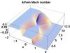 |
Fig. 3 Constructed Mach number profile. |
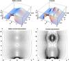 |
Fig. 4 Static (left) versus stationary (right) current (top) and its isocontours (bottom). For better visualization the current is plotted inversely and cut off at the numerical value of 2. The maximum at the origin approaches a numerical value of 6. |
Starting from the MHS equilibrium configuration for the flux function and its corresponding current distribution (see Sect. 3.1), we applied the mapping defined by the Mach number profile. The resulting current and its isocontour lines are displayed in the upper and lower right panels of Fig. 4. Obviously, the current distribution shows new features, which did not exist in the static case (left panels of Fig. 4). These are ring-like and crescent-shaped structures around both the lower, static configuration and the upper disconnected plasmoid. In both cases, these new current sheets are located outside but along the separatrix. In addition, inside the detached plasmoid, the current appears dome-like in the center, and two more current sheets (current “islands”) formed close to the separatrix. These new current structures (sheets, islands, maximum) are also visible in the isocontour plot. There, additional butterfly-like current islands appear in the vicinity of the X-point of the outer separatrix. The strongest currents can be recognized at the “Kan dipole”-region, because the increase of A and | BS | in the region of the pole of A results in strong currents already in the MHS-state. Applying the shear at the outer separatrix enforces this effect in particular at the bottom separatrix (in the vicinity of the photosphere), generating two additional current peaks. In the center of the static configuration (where MA was set to zero), the current structure has not changed. In contrast to the Grad-Shafranov theory, the stationary current isocontours do not (completely) resemble the field-line structure anymore.
To highlight the motion of the plasma, we display in Fig. 5 the x and y components of the normalized (with respect to density) plasma velocity field. The y component shows that in the outside regions it is always positive, in agreement with an upstream behavior of the flow on the open field-lines. The clockwise rotational flow of the plasma within the upper plasmoid is obvious from the y component of the flow being positive on the left side of the plasmoid, and negative on the right side. The x component of the flow is generally very small with a wavy structure due to the curved open field-lines in the vicinity of the outer separatrix. Only the circular flow inside the upper plasmoid has slightly higher velocity.
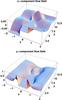 |
Fig. 5 x and y components of the plasma flow field. |
In summary, from an initially smooth current distribution our applied mapping created a new distribution, which shows multiple current filaments that can be regarded as current fragmentation.
 |
Fig. 6 Mach number profile (top), transformed inverse current density (middle) and its isocontours (bottom), for a narrower intrinsic current sheet with Ab = 0.01 and an intrinsically structured plasmoid with fp ≠ 1. |
4. Discussion
The results shown in the previous section serve as an illustration. There, the width of the current sheet, prescribed by the parameter Ab, was set to a value of 0.1, which resulted in pure, crescent-shaped current sheet structures. However, decreasing the value of Ab, i.e., steepening the Mach number profile and shrinking the width of the current sheet resulted in additional fragmentation of the crescent-shaped current sheet into several strong current peaks, as shown in the middle panel of Fig. 6 for which Ab was set to 0.01. For better visualization the current was cut at the numerical value of ten. From these results we may thus conclude that fragmentation is enforced when reaching smaller scales of the shear flows. Furthermore, fragmentation of the flux rope’s current density profile occurs when the parameter fp is different from 1. In the example depicted in Fig. 6 we used fp = 1−0.1sin [1/(A2 + 0.01)] and f = 1. The corresponding Mach number profile, which now already shows a small-scale structure imprinted on the plasmoid, is shown in the top panel of Fig. 6. The fine-structure obtained in the transformed current is obvious from both the current density profile and its isocontours (bottom panel of Fig. 6). For better visualization we also show in Fig. 7 a high-resolution zoom of the isocontours and the inverse current density for the same model parameters as in Fig. 6. The zoomed region contains the left side of the plasmoid. The plot of the isocontours demonstrates that the topology of the current isolines is much more complex than the one of the flux function isolines, i.e., the magnetic-field lines. The bottom panel of Fig. 7 displays the comparison between the static (dashed lines) and the stationary, fragmented current density (solid line) along the y-axis within the plasmoid region for x = −0.4. This plot highlights the strong spatial variation of the stationary current density, which shows steep gradients that imply fragmentation of the initially smooth current sheet. This relatively simple example stresses that to achieve fragmentation on much smaller scales, it is essential to use a Mach number profile, which is much more complex and contains highly alternating structures, e.g., in the form of saw-tooth-like or other oscillating functions. Furthermore, every Mach number profile could in principle successively and infinitely be refined by, e.g., an iterative scheme of the form f((MA)n) = (MA)n + 1. Such an iterative mapping can be performed because (MA)n is constant along the field lines, so every regular function or mapping has to be constant on the field lines as well. These iterations define fractal structures and hence demonstrate the fractal nature of MHD. The concept of fragmentation in the frame of ideal MHD remains valid down to length scales of 100 m to ~5 m for conditions typical for the solar corona. The value of ~5 m thereby corresponds to the ion inertial length, defined as the ratio of the speed of light and the ion plasma frequency. On length scales similar to and shorther than the ion inertial length, either the Hall-MHD or the two-fluid MHD needs to be applied.
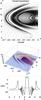 |
Fig. 7 High-resolution zoom into the plasmoid region for the same model as in Fig. 6. Shown are the isocontours (top), the transformed inverse current density (middle), and a cut through the current density at x = −0.4 (bottom) for the stationary (jz, solid) and the static case (jzs, dashed). |
In our analysis we ignored resistive or nonideal effects to guarantee the existence of plausible stationary flows. However, the presence of nonideal terms, particularly in the shape of a resistivity on the right-hand side of Ohm’s law, does not automatically imply the nonexistence of stationary solutions. The inclusion of a resistivity, η, such that ∇ × (ηj) = 0, supports stationary nonideal MHD flows and hence the existence of ideal equilibria. The stationarity of Maxwell equations in 2D demands that the electric-field component Ez = ηjz is constant. As Ez is at the same time the reconnection rate, this implies that the reconnection rate is independent of the resistivity (e.g., Knoll & Chacón 2006). Consequently, even if, as in our case, the flows are field-aligned and steady-state, these MHD flows can be regarded as an analogy to steady-state reconnection solutions with constant reconnection rate. The existence of resistive steady states with field-aligned flows and reasonable resistivity profiles has been shown by Throumoulopoulos & Tasso (2000, 2003). Under such conditions in our 2D case, Ohmic heating of the plasma is directly proportional to jz and occurs everywhere where filamentation or fragmentation takes place and could in principle contribute (at least partially) to the heating of the corona.
Although we had limited our analysis to a pure 2D configuration, the transformation technique is valid in all dimensions because it is based on vector analysis identities. Therefore, starting from a 3D MHS equilibrium, the mapping would deliver current fragmentation also in 3D. However, to find suitable MHS equilibria as starting configurations is a difficult task, hence pre-computed fully 3D MHS equilibria are so far rare. MHS equilibria for laminar flows and magnetic fields have been constructed by, e.g., Petrie & Neukirch (1999), which might serve as starting points for a future 3D analysis.
5. Conclusions
Observations of the solar atmosphere with increasing spatial resolution reveal that the atmosphere is highly structured or fragmented. Hence, the mechanisms initiating the formation of small-scale structures, such as jets, flares, and plasmoids, which typically occur as a result of magnetic reconnection processes of current sheets, must be inherently fractal.
Although solutions of the MHD equations pretend that physical parameters, such as the magnetic field or the current, are smooth on large scales, they do not necessarily have to be smooth on small scales. This is shown by our analysis, in which, starting from an MHS equilibrium with a smooth current distribution for a stationary plasmoid configuration, we obtained a current structure displaying steep gradients, i.e., strong spatial variations of the current density, as well as an internally fragmented plasmoid, depending on the initially chosen Mach number profile. Hence, pure MHD equilibria are able to display intrinsic fine structure, which can serve as the seeds for instabilities, i.e., as “secondary instabilities” (see, e.g., Pegoraro et al. 2010), and therefore as triggering mechanisms for second-generation current fragmentation.
Because the MHD equations are scale-free, our results are valid not only for the global flare scale, but also for scales close to dissipation scales.
As a natural next step, our stationary equilibrium configuration should be implemented into MHD simulations as the starting configuration, to see and test the onset of instabilities and the time-dependent evolution of the resulting additional current fragmentation.
A restriction to pure 2D is justified, because it enhances the clarity of the representation of the fragmentation process. Our studies are aimed at the fragmentation of the isocontours of the current density jz.
In dynamical flare scenarios, the plasma within the closed arcade structure tends to flow downwards, i.e. back to the surface because of plasma cooling, which forces the arcade structure to shrink. However, our model aims at studying the post-eruptive flare phase, in which the photospheric layers (i.e., the arcade structures at the bottom of our configuration) are back in static equilibrium (see, e.g., Wang et al. 2012).
Acknowledgments
We thank the anonymous referee for useful comments and suggestions on the draft. This research made use of the NASA Astrophysics Data System (ADS). D.H.N. and M.K. acknowledge financial support from GA ČR under grant number 13-24782. M.K. also acknowledges financial support from GA ČR under grant number P209/12/0103. The Astronomical Institute Ondřejov is supported by the project RVO:67985815.
References
- Bandle, C. 1975, Archive for Rational Mechanics and Analysis, 58, 219 [NASA ADS] [CrossRef] [Google Scholar]
- Bárta, M., Karlický, M., & Žemlička, R. 2008a, Sol. Phys., 253, 173 [NASA ADS] [CrossRef] [Google Scholar]
- Bárta, M., Vršnak, B., & Karlický, M. 2008b, A&A, 477, 649 [NASA ADS] [CrossRef] [EDP Sciences] [Google Scholar]
- Bárta, M., Büchner, J., & Karlický, M. 2010, Adv. Space Res., 45, 10 [NASA ADS] [CrossRef] [Google Scholar]
- Bárta, M., Büchner, J., Karlický, M., & Skála, J. 2011, ApJ, 737, 24 [NASA ADS] [CrossRef] [Google Scholar]
- Becker, U., Neukirch, T., & Schindler, K. 2001, J. Geophys. Res., 106, 3811 [NASA ADS] [CrossRef] [Google Scholar]
- Bennett, W. H. 1934, Phys. Rev., 45, 890 [NASA ADS] [CrossRef] [Google Scholar]
- Birn, J., Sommer, R., & Schindler, K. 1975, Ap&SS, 35, 389 [NASA ADS] [CrossRef] [Google Scholar]
- Birn, J., Sommer, R. R., & Schindler, K. 1977, J. Geophys. Res., 82, 147 [NASA ADS] [CrossRef] [Google Scholar]
- Birn, J., Goldstein, H., & Schindler, K. 1978, Sol. Phys., 57, 81 [NASA ADS] [CrossRef] [Google Scholar]
- Bogoyavlenskij, O. I. 2000, Phys. Rev. E, 62, 8616 [NASA ADS] [CrossRef] [Google Scholar]
- Bogoyavlenskij, O. I. 2001, Phys. Lett. A, 291, 256 [NASA ADS] [CrossRef] [Google Scholar]
- Bogoyavlenskij, O. I. 2002, Phys. Rev. E, 66, 056410 [NASA ADS] [CrossRef] [Google Scholar]
- Cargill, P. 2013, Nature, 493, 485 [NASA ADS] [CrossRef] [Google Scholar]
- Cirtain, J. W., Golub, L., Winebarger, A. R., et al. 2013, Nature, 493, 501 [NASA ADS] [CrossRef] [Google Scholar]
- Contopoulos, J. 1996, ApJ, 460, 185 [NASA ADS] [CrossRef] [Google Scholar]
- Eyink, G. L. 2011, Phys. Rev. E, 83, 056405 [NASA ADS] [CrossRef] [Google Scholar]
- Gebhardt, U., & Kiessling, M. 1992, Phys. Fluids B, 4, 1689 [NASA ADS] [CrossRef] [Google Scholar]
- Goedbloed, J. P., & Lifschitz, A. 1997, Phys. Plasmas, 4, 3544 [Google Scholar]
- Harris, E. G. 1962, Il Nuovo Cimento, 23, 115 [Google Scholar]
- Kan, J. R. 1973, J. Geophys. Res., 78, 3773 [NASA ADS] [CrossRef] [Google Scholar]
- Karlický, M. 2004, A&A, 417, 325 [NASA ADS] [CrossRef] [EDP Sciences] [Google Scholar]
- Karlický, M., & Bárta, M. 2011, ApJ, 733, 107 [NASA ADS] [CrossRef] [Google Scholar]
- Karlický, M., Fárník, F., & Mészárosová, H. 2002, A&A, 395, 677 [NASA ADS] [CrossRef] [EDP Sciences] [Google Scholar]
- Karlický, M., Bárta, M., & Nickeler, D. 2012, A&A, 541, A86 [NASA ADS] [CrossRef] [EDP Sciences] [Google Scholar]
- Kliem, B., Karlický, M., & Benz, A. O. 2000, A&A, 360, 715 [NASA ADS] [Google Scholar]
- Knoll, D. A., & Chacón, L. 2006, Phys. Plasmas, 13, 032307 [NASA ADS] [CrossRef] [Google Scholar]
- Konz, C., Wiechen, H., & Lesch, H. 2000, Phys. Plasmas, 7, 5159 [Google Scholar]
- Kowal, G., Lazarian, A., Vishniac, E. T., & Otmianowska-Mazur, K. 2009, ApJ, 700, 63 [NASA ADS] [CrossRef] [Google Scholar]
- Lazarian, A., & Vishniac, E. T. 1999, ApJ, 517, 700 [NASA ADS] [CrossRef] [Google Scholar]
- Loureiro, N. F., Schekochihin, A. A., & Cowley, S. C. 2007, Phys. Plasmas, 14, 100703 [NASA ADS] [CrossRef] [Google Scholar]
- Lüst, R., & Schlüter, A. 1957, Zeitschrift Naturforschung Teil A, 12, 850 [NASA ADS] [Google Scholar]
- Magara, T., Mineshige, S., Yokoyama, T., & Shibata, K. 1996, ApJ, 466, 1054 [NASA ADS] [CrossRef] [Google Scholar]
- Nickeler, D., & Fahr, H. J. 2001, in The Outer Heliosphere: The Next Frontiers, eds. K. Scherer, H. Fichtner, H. J. Fahr, & E. Marsch, 57 [Google Scholar]
- Nickeler, D. H., & Fahr, H.-J. 2005, Adv. Space Res., 35, 2067 [NASA ADS] [CrossRef] [Google Scholar]
- Nickeler, D. H., & Fahr, H.-J. 2006, Adv. Space Res., 37, 1292 [NASA ADS] [CrossRef] [Google Scholar]
- Nickeler, D. H., & Wiegelmann, T. 2010, Ann. Geophys., 28, 1523 [NASA ADS] [CrossRef] [Google Scholar]
- Nickeler, D. H., & Wiegelmann, T. 2012, Ann. Geophys., 30, 545 [NASA ADS] [CrossRef] [Google Scholar]
- Nickeler, D. H., Goedbloed, J. P., & Fahr, H.-J. 2006, A&A, 454, 797 [NASA ADS] [CrossRef] [EDP Sciences] [Google Scholar]
- Ohyama, M., & Shibata, K. 1998, ApJ, 499, 934 [NASA ADS] [CrossRef] [Google Scholar]
- Pegoraro, F., Califano, F., Faganello, M., & Tenerani, A. 2010, in AIP Conf. Ser., 1242, eds. G. Bertin, F. de Luca, G. Lodato, R. Pozzoli, & M. Romé, 89 [Google Scholar]
- Petrie, G. J. D., & Neukirch, T. 1999, Geophys. Astrophys. Fluid Dynam., 91, 269 [NASA ADS] [CrossRef] [Google Scholar]
- Schindler, K. 1972, in Earth’s Magnetospheric Processes, ed. B. M. McCormac, Astrophys. Space Sci. Lib., 32, 200 [Google Scholar]
- Schindler, K. 1979, Space Sci. Rev., 23, 365 [NASA ADS] [CrossRef] [Google Scholar]
- Schmid-Burgk, J. 1967, ApJ, 149, 727 [NASA ADS] [CrossRef] [Google Scholar]
- Shafranov, V. D. 1958, Sov. J. Exp. Theoret. Phys., 6, 545 [NASA ADS] [Google Scholar]
- Shibata, K. 2012a, in EGU General Assembly Conference Abstracts, 14, eds. A. Abbasi, & N. Giesen, 3226 [Google Scholar]
- Shibata, K. 2012b, in 39th COSPAR Scientific Assembly. Held 14–22 July, in Mysore, India, Abstract B0.5-3-12, COSPAR Meeting, 39, 1785 [Google Scholar]
- Shibata, K., & Tanuma, S. 2001, Earth, Planets, and Space, 53, 473 [Google Scholar]
- Throumoulopoulos, G. N., & Tasso, H. 2000, J. Plasma Phys., 64, 601 [NASA ADS] [CrossRef] [Google Scholar]
- Throumoulopoulos, G. N., & Tasso, H. 2003, Phys. Plasmas, 10, 2382 [NASA ADS] [CrossRef] [Google Scholar]
- Tsinganos, K. C. 1981, ApJ, 245, 764 [NASA ADS] [CrossRef] [Google Scholar]
- Uzdensky, D. A., Loureiro, N. F., & Schekochihin, A. A. 2010, Phys. Rev. Lett., 105, 235002 [NASA ADS] [CrossRef] [Google Scholar]
- Wang, S., Liu, C., & Wang, H. 2012, ApJ, 757, L5 [NASA ADS] [CrossRef] [Google Scholar]
- Wiechen, H., Birk, G. T., & Lesch, H. 1998, Phys. Plasmas, 5, 3732 [NASA ADS] [CrossRef] [Google Scholar]
- Wiegelmann, T., & Schindler, K. 1995, Geophys. Res. Lett., 22, 2057 [NASA ADS] [CrossRef] [Google Scholar]
- Wiegelmann, T., Schindler, K., & Neukirch, T. 1998, Sol. Phys., 180, 439 [NASA ADS] [CrossRef] [Google Scholar]
Appendix A: Proof of theorem
In Sect. 3.2.3 we claimed that for a given j Eq. (32) has in general no formal solution. One may argue that it is always possible to reduce Eq. (32) to an ordinary differential equation for α as a function of A. Here we show that this is indeed not the case, because the solution to any such differential equation returns the original form of the equation.
An equivalent representation of the current transformation Eq. (32) would be to use instead of the coordinates x and y the flux function A and the arc length s along a field line, or instead of s one of the coordinates x and y. The choice of such a representation has pure mathematical reasons: Eq. (32) should present an ordinary differential equation for α, and α itself should depend only on one single coordinate A. But the nonconstant coefficients of α′ are depending on two coordinates. The choice of a coordinate system that includes A as one of the coordinates enables us to formulate a constraint for which current distributions j the Eq. (32) is really an ordinary differential equation for α as a function of A.
As long as A is locally monotonic,
 usually
depends explicitely on the flux function A and the arc length
s along a field line as coordinates equivalent to x,y
in 2D, i.e.
usually
depends explicitely on the flux function A and the arc length
s along a field line as coordinates equivalent to x,y
in 2D, i.e.  etc.
etc.
Taking the function j(A,s) as a constraint for the MHD
system, one has to solve a partial differential equation in A,s or
x,y. The special shape  (A.1)is a strong
restriction for every prescribed current (function)
j(A,s). How to solve it correctly for any arbitrarily
prescribed j(A,s)? The problem is caused by the fact
that Eq. (A.1) is an equation defining or
rather determining j(A,s) from a given transformation.
Therefore, to prescribe α′(A) to calculate
j(A,s) seems to be the most consequent and logical
method.
(A.1)is a strong
restriction for every prescribed current (function)
j(A,s). How to solve it correctly for any arbitrarily
prescribed j(A,s)? The problem is caused by the fact
that Eq. (A.1) is an equation defining or
rather determining j(A,s) from a given transformation.
Therefore, to prescribe α′(A) to calculate
j(A,s) seems to be the most consequent and logical
method.
Nevertheless, an inverse method for calculating the transformation α(A) or rather α′(A) from the transformation equation for the current (Eq. (A.1)) would have great advantages, because it would make it possible to generate current fragmentation and strong current-sheets of arbitrary, “turbulent” structure, needed to induce magnetic reconnection or general plasma instabilities.
However, there are several obstacles to use an inverse method. First, it will be
difficult to express  as
as
 , at least analytically.
Second, one has to assume a special dependence of the current density
j(A,s) to fulfill Eq. (A.1). But any “arbitrary” choice of
j(A,s) can overdetermine this ordinary (mixed)
differential equation, because the function j(A,s) must
be “separable” in the sense of Eq. (A.1).
, at least analytically.
Second, one has to assume a special dependence of the current density
j(A,s) to fulfill Eq. (A.1). But any “arbitrary” choice of
j(A,s) can overdetermine this ordinary (mixed)
differential equation, because the function j(A,s) must
be “separable” in the sense of Eq. (A.1).
An equivalent formulation of Eq. (A.1)
can be found by eliminating all terms and derivatives of α. This results
in the following differential equation  (A.2)which represents a
constraint for j(A,s).
(A.2)which represents a
constraint for j(A,s).
Because any formal integration of Eq. (A.2) leads automatically back to Eq. (A.1), Eq. (A.2) is only a necessary condition, testing or proving if any considered current density j(A,s) enables the calculation of the transformation α′(A) from Eq. (A.1).
The same integration procedure as in Eq. (33) leading to Eq. (34) could
basically also be performed for completely 2D equilibria, which are not asymptotically 1D.
The only restriction is again the integrability condition: to guarantee the existence of
an allowed transformation (to be precise, α′ should be an
explicit function of A only), the condition  must
be valid. Here C0 is an explicit function of
s only,
must
be valid. Here C0 is an explicit function of
s only,  is an
explicit function of A, and BS and
j are explicit functions of A and s.
The partial differential equation Eq. (A.3) is now only of first order, concerning the
∂/∂s derivative, in contrast to the
Eq. (A.2), but the problem of
integrability can also neither be eliminated nor solved in this way. Conversely, the
procedure in Sect. 3.2.3 fulfills the integrability
condition Eq. (A.3) automatically, because
it is an asymptotical 1D problem.
is an
explicit function of A, and BS and
j are explicit functions of A and s.
The partial differential equation Eq. (A.3) is now only of first order, concerning the
∂/∂s derivative, in contrast to the
Eq. (A.2), but the problem of
integrability can also neither be eliminated nor solved in this way. Conversely, the
procedure in Sect. 3.2.3 fulfills the integrability
condition Eq. (A.3) automatically, because
it is an asymptotical 1D problem.
All Figures
|
Fig. 1 Sketch of a magnetic configuration of a solar flare with plasmoids formed via magnetic reconnection processes. |
| In the text | |
|
Fig. 2 Field lines for the Kan magnetotail (top), the periodic sheet pinch or periodic Harris sheet (middle), and the combined one (bottom) that serves as our initial MHS equilibrium. |
| In the text | |
|
Fig. 3 Constructed Mach number profile. |
| In the text | |
|
Fig. 4 Static (left) versus stationary (right) current (top) and its isocontours (bottom). For better visualization the current is plotted inversely and cut off at the numerical value of 2. The maximum at the origin approaches a numerical value of 6. |
| In the text | |
|
Fig. 5 x and y components of the plasma flow field. |
| In the text | |
|
Fig. 6 Mach number profile (top), transformed inverse current density (middle) and its isocontours (bottom), for a narrower intrinsic current sheet with Ab = 0.01 and an intrinsically structured plasmoid with fp ≠ 1. |
| In the text | |
|
Fig. 7 High-resolution zoom into the plasmoid region for the same model as in Fig. 6. Shown are the isocontours (top), the transformed inverse current density (middle), and a cut through the current density at x = −0.4 (bottom) for the stationary (jz, solid) and the static case (jzs, dashed). |
| In the text | |
Current usage metrics show cumulative count of Article Views (full-text article views including HTML views, PDF and ePub downloads, according to the available data) and Abstracts Views on Vision4Press platform.
Data correspond to usage on the plateform after 2015. The current usage metrics is available 48-96 hours after online publication and is updated daily on week days.
Initial download of the metrics may take a while.