| Issue |
A&A
Volume 543, July 2012
|
|
|---|---|---|
| Article Number | A136 | |
| Number of page(s) | 8 | |
| Section | Cosmology (including clusters of galaxies) | |
| DOI | https://doi.org/10.1051/0004-6361/201219590 | |
| Published online | 11 July 2012 | |
Mixing of blackbodies: entropy production and dissipation of sound waves in the early Universe
1
Max Planck Institut für Astrophysik,
Karl-Schwarzschild-Str. 1,
85741
Garching,
Germany
e-mail: This email address is being protected from spambots. You need JavaScript enabled to view it.
2
Space Research Institute, Russian Academy of Sciences,
Profsoyuznaya
84/32, 117997
Moscow,
Russia
3
Institute for Advanced Study, Einstein Drive, Princeton, New
Jersey
08540,
USA
4
Canadian Institute for Theoretical Astrophysics,
60 St George Street,
Toronto, ON
M5S 3H8,
Canada
Received:
13
May
2012
Accepted:
8
June
2012
Abstract
Mixing of blackbodies with different temperatures creates a spectral distortion which, at lowest order, is a y-type distortion, indistinguishable from the thermal y-type distortion produced by the scattering of cosmic microwave background (CMB) photons by hot electrons residing in clusters of galaxies. This process occurs in the radiation-pressure dominated early Universe, when the primordial perturbations excite standing sound waves on entering the sound horizon. Photons from different phases of the sound waves, having different temperatures, diffuse through the electron-baryon plasma and mix together. This diffusion, with the length defined by Thomson scattering, dissipates sound waves and creates spectral distortions in the CMB. Of the total dissipated energy, 2/3 raises the average temperature of the blackbody part of spectrum, while 1/3 creates a distortion of y-type. It is well known that at redshifts 105 ≲ z ≲ 2 × 10⁶, comptonization rapidly transforms y-distortions into a Bose-Einstein spectrum. The chemical potential of the Bose-Einstein spectrum is again 1/3 the value we would get if all the dissipated energy was injected into a blackbody spectrum but no extra photons were added. We study the mixing of blackbody spectra, emphasizing the thermodynamic point of view, and identifying spectral distortions with entropy creation. This allows us to obtain the main results connected with the dissipation of sound waves in the early Universe in a very simple way. We also show that mixing of blackbodies in general, and dissipation of sound waves in particular, leads to creation of entropy.
Key words: cosmic background radiation / cosmology: theory / early Universe
© ESO, 2012
1. Introduction
The cosmic microwave background (CMB) has a spectrum which is close to a blackbody with very high precision. COBE/FIRAS (Fixsen et al. 1996) constrained possible departures from a perfect blackbody to be ≲ 10-5 for y-type distortions, and the chemical potential was limited to |μ| ≲ 9 × 10⁻⁵. This observation immediately has an important consequence: there was a time in the history of the Universe when matter and radiation were in complete thermodynamic equilibrium with each other and any energy release at z ≲ 2 × 10⁶ was small.
In addition to being an almost perfect blackbody, the CMB is also isotropic, with
anisotropies of less than 10-3. The dominant component of the anisotropy is the
dipole caused by our peculiar motion. The anisotropies other than the dipole are at the
level of 10-5 and originate from the primordial fluctuations imprinted in the
initial conditions of the present expanding Universe. The radiation field seen by any
observer (or electrons in the hot gas in a cluster of galaxies/early Universe) will thus
consist of blackbodies having temperature that differs as a function of observation
direction. Scattering by electrons, averaging of the smaller scales within the beam of the
telescope or explicit averaging by a cosmologist, will thus inevitably mix these blackbodies
together. Mixing of blackbodies was first studied in detail by (Zeldovich et al. 1972) who showed that it creates a
y-type distortion, indistinguishable from the y-type
distortion created by interaction of the blackbody photons with hotter electrons (Zeldovich & Sunyaev 1969). Chluba & Sunyaev (2004) proved that at lowest order, this result
is valid for arbitrary temperature distributions and not just the Gaussian ones.
Comptonization of this initial y-type distortion converts it into a
Bose-Einstein spectrum or a μ-type distortion (Zeldovich & Sunyaev 1969; Chluba
et al. 2012b) for y ≳ 1, where the Compton
y-parameter is defined as the following integral over time
t:  , ne is
the electron number density, σT is the Thomson cross section,
c is the speed of light, kB is the
Boltzmann’s constant, Te is the electron temperature, and
me is the mass of electron (Kompaneets 1956; Zeldovich & Sunyaev
1969). The purpose of this paper is to study the mixing of blackbodies from a
statistical physics point of view. Amazingly, using basic thermodynamic relations, we arrive
at the main results connected with the dissipation of sound waves in the early Universe due
to shear viscosity and thermal conduction in a very simple manner. Some of these aspects are
also discussed in Chluba et al. (2012b).
, ne is
the electron number density, σT is the Thomson cross section,
c is the speed of light, kB is the
Boltzmann’s constant, Te is the electron temperature, and
me is the mass of electron (Kompaneets 1956; Zeldovich & Sunyaev
1969). The purpose of this paper is to study the mixing of blackbodies from a
statistical physics point of view. Amazingly, using basic thermodynamic relations, we arrive
at the main results connected with the dissipation of sound waves in the early Universe due
to shear viscosity and thermal conduction in a very simple manner. Some of these aspects are
also discussed in Chluba et al. (2012b).
2. Entropy of a Bose gas
The entropy density of a general distribution of a Bose gas (photons), which may or may not
be in equilibrium, is given by (Landau & Lifshitz
1980) ![Mathematical equation: \begin{eqnarray} S&&=\int \id\nu \frac{8\pi \nu^2}{c^3}\left[(1+n)\ln(1+n)-n\ln(n)\right]\nonumber\\ &&=8\pi\left(\frac{\kB T }{h c}\right)^3\int x^2\left[(1+n)\ln(1+n)-n\ln(n)\right]~\id x \end{eqnarray}](/articles/aa/full_html/2012/07/aa19590-12/aa19590-12-eq20.png) (1)where
(1)where
 is the density of available states in the frequency interval dν, and for
photons the degeneracy g = 2, h is Planck’s constant,
is the density of available states in the frequency interval dν, and for
photons the degeneracy g = 2, h is Planck’s constant,
 is the photon occupation number and Eν is the
energy density of photons per unit frequency. We have changed variables to dimensionless
frequency
x = hν/(kBT)
defined with respect to a reference temperature T in the second line. For a
blackbody spectrum at temperature T with
n = nPl(x) ≡ 1/(ex − 1),
we obtain
is the photon occupation number and Eν is the
energy density of photons per unit frequency. We have changed variables to dimensionless
frequency
x = hν/(kBT)
defined with respect to a reference temperature T in the second line. For a
blackbody spectrum at temperature T with
n = nPl(x) ≡ 1/(ex − 1),
we obtain  , where the last line
defines the radiation constant aR.
, where the last line
defines the radiation constant aR.
Now let us add a small spectral distortion δn to the Planck spectrum so
that the total occupation number is
n = nPl(1 + δn/nPl),
where δn/nPl ≪ 1. Expanding
the expression for entropy up to first order in
δn/nPl and ignoring the
higher order terms, we get
S = Spl + δS, where
δS is the entropy density added/subtracted due to the spectral distortion
and is given by, ![Mathematical equation: \begin{eqnarray} \delta S&&\approx 8\pi\left(\frac{\kB T }{h c}\right)^3\int x^2\left[\ln(1+\npl)-\ln(\npl)\right]\delta n~~\id x\nonumber\\ \label{noneqent}&&=8\pi\left(\frac{\kB T }{h c}\right)^3\int x^3\delta n~~\id x\equiv\frac{\delta Q}{\kB T}, \end{eqnarray}](/articles/aa/full_html/2012/07/aa19590-12/aa19590-12-eq38.png) (2)where
δQ is the energy density in the distortion. Thus for small distortions,
the classic thermodynamical formula for the change in the equilibrium entropy due to
addition/subtraction of energy remains valid even in non-equilibrium. We note in particular
that, at first order in distortions, the entropy does not depend on the shape of the
distortion but only on the total energy density in the distortion. This means that the
process of comptonization, which converts an initial y-type distortion to a
μ-type distortion, in the absence of any additional heating/cooling, does
not change the entropy of the photon gas at first order. The factor of
kB in Eq. (2)just converts temperature from Kelvin to energy units to make entropy
dimensionless. As an example, we can calculate the entropy produced during cosmological
recombination, when ~5 energetic recombination photons are produced per hydrogen atom
(Chluba & Sunyaev 2006). Adding up the
energy in the recombination spectrum (Rubiño-Martín et al.
2008), we get
δSrecombination ~ δQrecombination/(kBTCMB) ~ 9 × 10⁻⁶/cm3
today, compared with entropy density of 1478/cm3 in the
blackbody part of CMB with temperature TCMB = 2.725 K.
(2)where
δQ is the energy density in the distortion. Thus for small distortions,
the classic thermodynamical formula for the change in the equilibrium entropy due to
addition/subtraction of energy remains valid even in non-equilibrium. We note in particular
that, at first order in distortions, the entropy does not depend on the shape of the
distortion but only on the total energy density in the distortion. This means that the
process of comptonization, which converts an initial y-type distortion to a
μ-type distortion, in the absence of any additional heating/cooling, does
not change the entropy of the photon gas at first order. The factor of
kB in Eq. (2)just converts temperature from Kelvin to energy units to make entropy
dimensionless. As an example, we can calculate the entropy produced during cosmological
recombination, when ~5 energetic recombination photons are produced per hydrogen atom
(Chluba & Sunyaev 2006). Adding up the
energy in the recombination spectrum (Rubiño-Martín et al.
2008), we get
δSrecombination ~ δQrecombination/(kBTCMB) ~ 9 × 10⁻⁶/cm3
today, compared with entropy density of 1478/cm3 in the
blackbody part of CMB with temperature TCMB = 2.725 K.
In the rest of the paper we will measure frequency and temperature in energy units and set c = h = kB = 1 unless explicitly specified in definitions of other constants.
3. Mixing of blackbodies
Since the blackbody radiation is an equilibrium distribution for photons it is described by
a single parameter, the temperature T. In addition, if we specify a second
thermodynamic quantity such as volume V, we can calculate any other
thermodynamic quantity such as entropy or internal energy. The spectrum is described by the
well known Planck function, and the energy density per unit frequency and total energy
density integrated over frequency can be written as,
 (3)The
number density of photons is given by
N = bRT3 where
(3)The
number density of photons is given by
N = bRT3 where
 ,
ζ is the Riemann zeta function with ζ(3) ≈ 1.20206. We
can also calculate the entropy density and it is given by
S = 4E/(3T) = (4/3)aRT3.
For the CMB with TCMB = 2.725 K ± 1 mK (Fixsen & Mather 2002) we have energy density
ECMB = 0.26 eV/cm3, number
density NCMB = 411/cm3 and entropy
density SCMB = 1478/cm3. For
simplicity, we will consider mixing of two blackbodies below, but the derivation and the
results are trivially generalized to an ensemble of arbitrary number of blackbodies by just
replacing the average of quantities over two blackbodies with the appropriate average over
the whole ensemble.
,
ζ is the Riemann zeta function with ζ(3) ≈ 1.20206. We
can also calculate the entropy density and it is given by
S = 4E/(3T) = (4/3)aRT3.
For the CMB with TCMB = 2.725 K ± 1 mK (Fixsen & Mather 2002) we have energy density
ECMB = 0.26 eV/cm3, number
density NCMB = 411/cm3 and entropy
density SCMB = 1478/cm3. For
simplicity, we will consider mixing of two blackbodies below, but the derivation and the
results are trivially generalized to an ensemble of arbitrary number of blackbodies by just
replacing the average of quantities over two blackbodies with the appropriate average over
the whole ensemble.
3.1. y-type distortion
If we mix blackbody spectra with different temperature, the resultant spectrum is not
blackbody and at lowest order the distortion is given by a y-type
spectrum (Zeldovich et al. 1972)1. This can be seen immediately by Taylor expanding the photon
intensity or equivalently the occupation number n of a blackbody at a
temperature T + ΔT about the average temperature
T and take the average (ensemble or spatial) keeping terms up to second
order in ΔT/T, ![Mathematical equation: \begin{eqnarray} &&\left<\npl(T+\Delta T)\right>\equiv \left<\frac{1}{{\rm e}^{\frac{\nu}{(T+\Delta T)}}-1}\right>\nonumber\\ \approx &&\left<\npl(T)+\ln\left[1+\frac{\Delta T}{T}\right]\frac{\partial \npl}{\partial \ln[T]}+\frac{1}{2}\left(\ln\left[1+\frac{\Delta T}{T}\right]\right)^2\frac{\partial^2 \npl}{\partial (\ln[T])^2}\right>\nonumber\\ =&&\npl(T)+\left(\left<\frac{\Delta T}{T}\right>\!+\!\left<\left(\frac{\Delta T}{T}\right)^2\right>\right)T\frac{\partial \npl}{\partial T}\!+\!\frac{1}{2}\left<\left(\frac{\Delta T}{T}\right)^2\right>T^4\frac{\partial }{\partial T}\frac{1}{T^2}\frac{\partial \npl}{\partial T}\nonumber\\ \label{taylor} =&&\npl\left[T\left(1+\left<\left(\frac{\Delta T}{T}\right)^2\right>\right)\right]+\frac{1}{2}Y(x)\left<\left(\frac{\Delta T}{T}\right)^2\right>, \end{eqnarray}](/articles/aa/full_html/2012/07/aa19590-12/aa19590-12-eq59.png) (4)where
we have used
(4)where
we have used  . The first term in the last line
is simply a blackbody with temperature
Tnew = T [1 + (ΔT/T)2] > T,
and
. The first term in the last line
is simply a blackbody with temperature
Tnew = T [1 + (ΔT/T)2] > T,
and  (5)is
the y-type spectrum with
x = ν/T (Zeldovich & Sunyaev 1969) with the magnitude of
distortion given by
(5)is
the y-type spectrum with
x = ν/T (Zeldovich & Sunyaev 1969) with the magnitude of
distortion given by  . The average spectrum with
y-type distortion for average of two blackbodies with temperature
T ± ΔT is shown in Fig. 1. Figure 2 shows the same spectra but in
terms of the effective temperature defined by
n(ν) = 1/(eν/Teff(ν) − 1),
which for small distortions can be written, at linear order, as
Teff(x) = T + T[(1−e−x)/x]δn/n.
We note that in the Rayleigh-Jeans limit, intensity is proportional to temperature, and
thus the average of blackbody spectra just gives the spectrum at average temperature
T, and Teff → T. An
important property of y-type distortion is that it represents pure
redistribution of photons in the spectrum due to addition of energy but conserves photon
number. Thus
. The average spectrum with
y-type distortion for average of two blackbodies with temperature
T ± ΔT is shown in Fig. 1. Figure 2 shows the same spectra but in
terms of the effective temperature defined by
n(ν) = 1/(eν/Teff(ν) − 1),
which for small distortions can be written, at linear order, as
Teff(x) = T + T[(1−e−x)/x]δn/n.
We note that in the Rayleigh-Jeans limit, intensity is proportional to temperature, and
thus the average of blackbody spectra just gives the spectrum at average temperature
T, and Teff → T. An
important property of y-type distortion is that it represents pure
redistribution of photons in the spectrum due to addition of energy but conserves photon
number. Thus  and the above mentioned
decomposition of the spectrum into a blackbody part and y-distortion part
is unique and independent of gauge/reference frame, at order
δn/n, in the following sense: the
constraint
and the above mentioned
decomposition of the spectrum into a blackbody part and y-distortion part
is unique and independent of gauge/reference frame, at order
δn/n, in the following sense: the
constraint  on the spectral distortion
δn fixes the reference temperature of the blackbody part of the
spectrum used to define the variable x and δn as a
function of the variable x is gauge independent2.
on the spectral distortion
δn fixes the reference temperature of the blackbody part of the
spectrum used to define the variable x and δn as a
function of the variable x is gauge independent2.
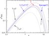 |
Fig. 1 Average of blackbodies of temperature T + ΔT and T − ΔT creates a new spectrum marked “Average(Y)” which is different from blackbody spectrum marked with temperature T. The average spectrum is just the usual y-type distortion with respect to a new blackbody at temperature T [1 + (ΔT/T)2] , with the two crossing at x = 3.83. At redshifts z ≳ 105 the average spectrum will comptonize to Bose-Einstein spectrum marked μ above. All three spectra, T [1 + (ΔT/T)2] , Average (Y), and μ, have the same number density of photons. Average/y-type spectrum and Bose-Einstein/μ-type spectrum also have the same energy density which is greater than the energy density in the blackbody spectrum with temperature T [1 + (ΔT/T)2] by 1/3 of the initial energy density excess over that of blackbody with temperature T. We have used linear order formulae to calculate the y and μ distortions in the figure but used a large value of ΔT/T to make differences between different curves visible. |
Without loss of generality, let us consider the superposition of two blackbody spectra
with temperatures
T1 = T + ΔT and
T2 = T − ΔT, with average
temperature T. The average initial energy density, number density and
entropy density of the two blackbodies is ![Mathematical equation: \begin{eqnarray} E_{\rm initial}&&=\frac{1}{2}\aR\left(T_1^4+T_2^4\right)\approx \aR T^4\left[1+6\left(\frac{\Delta T}{T}\right)^2\right]>\aR T^4\nonumber\\ N_{\rm initial}&&=\frac{1}{2}\bR\left(T_1^3+T_2^3\right)\approx \bR T^3\left[1+3\left(\frac{\Delta T}{T}\right)^2\right]>\bR T^3\nonumber\\ \label{initialeq} S_{\rm initial}&&=\frac{1}{2}\frac{4\aR}{3}\left(T_1^3+T_2^3\right)\approx \frac{4\aR}{3} T^3\left[1+3\left(\frac{\Delta T}{T}\right)^2\right]>\frac{4\aR}{3} T^3. \end{eqnarray}](/articles/aa/full_html/2012/07/aa19590-12/aa19590-12-eq80.png) (6)We
can calculate the final temperature of a blackbody having the same number density of
photons as the initial average
Ninitial
(6)We
can calculate the final temperature of a blackbody having the same number density of
photons as the initial average
Ninitial![Mathematical equation: \begin{eqnarray} T_{\rm final}=\left(\frac{N_{\rm initial}}{\bR}\right)^{1/3}\approx T\left[1+\left(\frac{\Delta T}{T}\right)^2\right]\cdot \end{eqnarray}](/articles/aa/full_html/2012/07/aa19590-12/aa19590-12-eq82.png) (7)This
is exactly the temperature, Tnew, of the blackbody we got by
averaging the intensity in Eq. (4). Thus
all the initial photons go into creating a blackbody with a higher
temperature. The entropy density of this new blackbody is also identical to the initial
average entropy density Sinitial because number density and
entropy density have the same T3 temperature dependence. The
energy density of the new blackbody is however given by,
(7)This
is exactly the temperature, Tnew, of the blackbody we got by
averaging the intensity in Eq. (4). Thus
all the initial photons go into creating a blackbody with a higher
temperature. The entropy density of this new blackbody is also identical to the initial
average entropy density Sinitial because number density and
entropy density have the same T3 temperature dependence. The
energy density of the new blackbody is however given by,
![Mathematical equation: \begin{eqnarray} E_{\rm final}&&=\aR T_{\rm final}^4 \approx \aR T^4\left[1+4\left(\frac{\Delta T}{T}\right)^2\right]<E_{\rm initial}. \end{eqnarray}](/articles/aa/full_html/2012/07/aa19590-12/aa19590-12-eq86.png) (8)In
fact we find
(8)In
fact we find 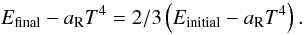 (9)This
result can also be obtained directly by multiplying Eq. (4)by ν3 and integrating over frequency.
Equation (4)also shows that the rest of
the initial energy, equal to
(9)This
result can also be obtained directly by multiplying Eq. (4)by ν3 and integrating over frequency.
Equation (4)also shows that the rest of
the initial energy, equal to 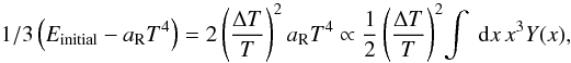 (10)goes
to the y-distortion with the magnitude of the distortion given by
(10)goes
to the y-distortion with the magnitude of the distortion given by
 . These results
were recently obtained in Chluba et al. (2012b)
using the Boltzmann equation. It is well known (Zeldovich
& Sunyaev 1969) that y-distortion of magnitude
yY decreases the brightness temperature of
radiation in the Rayleigh-Jeans part of the spectrum by an amount
−2yY which is equal to
. These results
were recently obtained in Chluba et al. (2012b)
using the Boltzmann equation. It is well known (Zeldovich
& Sunyaev 1969) that y-distortion of magnitude
yY decreases the brightness temperature of
radiation in the Rayleigh-Jeans part of the spectrum by an amount
−2yY which is equal to
 for the mixing
of blackbodies considered here. But we have also increased the magnitude of the brightness
temperature by same amount in the blackbody part of the spectrum, resulting in the
brightness temperature in the Rayleigh-Jeans part for the total spectrum which is equal to
the average temperature T of the initial blackbodies, as shown in
Figs. 1 and 2.
We can calculate the additional entropy in the final spectrum resulting from the mixing of
blackbodies using Eq. (2),
for the mixing
of blackbodies considered here. But we have also increased the magnitude of the brightness
temperature by same amount in the blackbody part of the spectrum, resulting in the
brightness temperature in the Rayleigh-Jeans part for the total spectrum which is equal to
the average temperature T of the initial blackbodies, as shown in
Figs. 1 and 2.
We can calculate the additional entropy in the final spectrum resulting from the mixing of
blackbodies using Eq. (2), 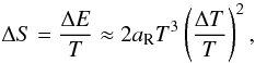 (11)where
 is
the energy in spectral distortion, i.e. deviation from the blackbody spectrum.
is
the energy in spectral distortion, i.e. deviation from the blackbody spectrum.
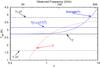 |
Fig. 2 Same as Fig. 1 but effective temperature Teff(ν) defined by n(ν) = 1/(eν/Teff(ν) − 1) is plotted. We have used linear order formulae to calculate the y and μ distortions in the figure but used a large value of ΔT/T = 0.4 to make differences between different curves visible. Average temperature T = 2.725 K. For Bose-Einstein spectrum we thus have, at linear order, Teff(x) = TBE − Tμ/x. For a general distortion δn/n (including y-type ) we have Teff(x) = T + T[(1−e−x)/x]δn/n. |
To summarize, mixing/averaging of blackbodies leads to a new spectrum which has a blackbody part at a temperature which is higher than the average temperature of initial blackbodies by ΔTnew = T(ΔT/T)2. This new blackbody has the same entropy as initial average entropy and the same number of photons but less energy. The remaining energy density appears as a y-type distortion, which is just a redistribution of the photons of the new blackbody spectrum. The y-distortion part can be identified with the increase in the entropy of the system (Eq. (11)), which is expected as there is an increase in disorder of the system.
3.2. μ-type distortion
We saw in the previous section that it is impossible to create a blackbody spectrum by
mixing/averaging blackbodies of different temperatures. The reason is that there is too
much energy density for the given number density of photons. However we can still create a
Bose-Einstein spectrum with a non zero chemical potential μ, which is the
spectrum we would get if the photons could again reach equilibrium while conserving energy
and number. It is straightforward to calculate the temperature and chemical potential of
the Bose-Einstein spectrum,
nBE = 1/(eν/TBE + μ − 1),
by equating the initial average photon number Ninitial and
energy density Einitial to the photon number
NBE and energy density EBE in a
Bose-Einstein spectrum, as is done in case of heating of CMB without adding additional
photons (Illarionov & Sunyaev 1975). In the
limit of small chemical potential, μ ≪ 1, with
TBE = Tnew(1 + tBE) ≈ T(1 + tBE + [ΔT/T] 2),tBE ≪ 1
we have (Illarionov & Sunyaev 1975)3![Mathematical equation: \begin{eqnarray} E_{\rm BE}&&\approx \aR T_{\rm BE}^4\left(1-1.1106 \mu \right)\nonumber\\ &&\approx \aR T^4\left(1+4 t_{\rm BE}+4\left(\frac{\Delta T}{T}\right)^2-1.1106 \mu \right)\nonumber\\ &&=E_{\rm initial}\approx \aR T^4\left[1+6\left(\frac{\Delta T}{T}\right)^2\right],\nonumber\\ N_{\rm BE}&\approx \bR T_{\rm BE}^3\left(1-1.3684 \mu \right)\nonumber\\ &&\approx \bR T^3\left(1 + 3 t_{\rm BE}+3\left(\frac{\Delta T}{T}\right)^2-1.3684 \mu \right)\nonumber\\ &&=N_{\rm initial}\approx \bR T^3\left[1+3\left(\frac{\Delta T}{T}\right)^2\right]\cdot \end{eqnarray}](/articles/aa/full_html/2012/07/aa19590-12/aa19590-12-eq107.png) (12)The
second equation, NBE = Ninitial,
directly gives us the relation
tBE = 1.3684μ/3 = μ/2.19.
Solving the system of equations for tBE and μ
in terms of ΔT/T, we get
(12)The
second equation, NBE = Ninitial,
directly gives us the relation
tBE = 1.3684μ/3 = μ/2.19.
Solving the system of equations for tBE and μ
in terms of ΔT/T, we get
![Mathematical equation: \begin{eqnarray} \mu&&=1.4\left[\frac{1}{3}\left(E_{\rm initial}-\aR T^4\right)\right]=2.8 \left(\frac{\Delta T}{T}\right)^2\nonumber\\ t_{\rm BE}&&=\frac{\mu}{2.19}=1.278\left(\frac{\Delta T}{T}\right)^2 \end{eqnarray}](/articles/aa/full_html/2012/07/aa19590-12/aa19590-12-eq111.png) (13)this
is exactly the result we will get if we add energy
(13)this
is exactly the result we will get if we add energy 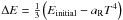 to
a blackbody with temperature Tnew while conserving the photon
number. We can thus write the deviation of the μ-type spectrum from the
blackbody with temperature Tnew:
to
a blackbody with temperature Tnew while conserving the photon
number. We can thus write the deviation of the μ-type spectrum from the
blackbody with temperature Tnew:
 (14)The
μ-type spectrum resulting from the average of two blackbodies is also
shown in Figs. 1 and 2. An important point to note here is that the Bose-Einstein spectrum is
uniquely fixed by energy density and number density constraints. In particular, the value
of the chemical potential μ is independent of any reference temperature
we may choose to define the dimensionless variable x. This is, of course,
the same value of μ we would get if we just comptonize the
y-type distortion of the previous section. The Bose-Einstein spectrum
and the chemical potential has however more fundamental origins in statistical physics,
compared to the y-type distortion, the shape of which originates in the
Compton scattering process or sum of Planck spectra. The μ-type results
of this section can thus be considered as the basis for our definitions of the spectral
distortion as pure redistribution of photons, and in particular of the 2:1 division of
initial energy in temperature perturbations into a blackbody part and a spectral
distortion part. Further justification is provided by the fact that with this definition,
the spectral distortion can also be identified with the entropy production.
(14)The
μ-type spectrum resulting from the average of two blackbodies is also
shown in Figs. 1 and 2. An important point to note here is that the Bose-Einstein spectrum is
uniquely fixed by energy density and number density constraints. In particular, the value
of the chemical potential μ is independent of any reference temperature
we may choose to define the dimensionless variable x. This is, of course,
the same value of μ we would get if we just comptonize the
y-type distortion of the previous section. The Bose-Einstein spectrum
and the chemical potential has however more fundamental origins in statistical physics,
compared to the y-type distortion, the shape of which originates in the
Compton scattering process or sum of Planck spectra. The μ-type results
of this section can thus be considered as the basis for our definitions of the spectral
distortion as pure redistribution of photons, and in particular of the 2:1 division of
initial energy in temperature perturbations into a blackbody part and a spectral
distortion part. Further justification is provided by the fact that with this definition,
the spectral distortion can also be identified with the entropy production.
One important difference from the heating of CMB usually considered, for example, in clusters of galaxies or due to decay of particles in the early Universe, is that in mixing of blackbodies, we are also adding photons (compared to a blackbody at initial average temperature). The additional photons are able to create a new blackbody at a higher temperature, which is impossible if the photon number density is kept constant.
Although we have derived the above formulae by considering only two blackbodies, they are applicable to an ensemble with arbitrary number of blackbodies by just replacing the average over two blackbodies (ΔT/T)2 with the average over the ensemble, ⟨ (ΔT/T)2 ⟩ .
4. Example: Mixing of the blackbodies in the observed CMB sky
One obvious and cleanest source of blackbodies of different temperatures is the CMB sky.
The temperature in different directions in the sky differs by ~10 μK
(Bennett et al. 1996; Komatsu et al. 2011) corresponding to the 10-5 spatial
fluctuations in the energy density of radiation/matter in the early Universe before
recombination4. Thus any telescope, due to finite
width of its beam, looking at the microwave sky will inevitably mix the spectra of
blackbodies of different temperature within the beam (Chluba
& Sunyaev 2004). In addition we may explicitly average the intensity over
the whole sky to achieve higher sensitivity and precision in the measurement of CMB spectrum
as is done, for example, by COBE (Fixsen et al. 1996)
and in the proposed experiment PIXIE (Kogut et al.
2011). The (angular) average amount of energy in CMB anisotropies is given by
(Chluba & Sunyaev 2004),
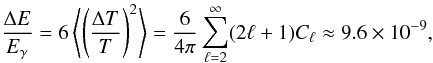 (15)where
Eγ is the energy density of CMB photons. One
third of this energy creates a y-distortion of magnitude
(15)where
Eγ is the energy density of CMB photons. One
third of this energy creates a y-distortion of magnitude
 .
The measured temperature from averaged intensity is also higher than the averaged
temperature TCMB by
.
The measured temperature from averaged intensity is also higher than the averaged
temperature TCMB by  accounting for the remaining
2/3 of energy in anisotropies. The increase in entropy in this mixing
is
accounting for the remaining
2/3 of energy in anisotropies. The increase in entropy in this mixing
is  .
.
In the above estimate we ignored the dipole which has been measured by COBE and WMAP (Bennett et al. 1996; Jarosik et al. 2011) to have an amplitude equal to 3.355 ± 0.008 mK corresponding to our peculiar motion v = 1.23 × 10⁻³. The average power from dipole is then 3C1/(4π) = v2/3. The resulting y distortion is v2/6 = 2.5 × 10⁻⁷ and increase in monopole temperature is v2/3 = 1.4 μK. The increase in entropy from the mixing of the CMB dipole on our sky is ΔS = 1.1 × 10⁻³/cm3.
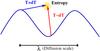 |
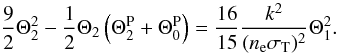
Fig. 3 Cartoon picture of mixing of blackbodies: photons from different phases of sound wave mix and create spectral distortion/entropy. |
5. Application: dissipation of sound waves in the early Universe
Before recombination, we have a tightly coupled plasma of radiation-electrons-baryons in
the early Universe. At high redshifts, both the energy density and pressure in the plasma
are dominated by radiation while at low redshifts, but before recombination, the baryon
energy density becomes important, although pressure is still dominated by radiation. Sound
speed in this relativistic plasma is therefore  and Jeans scale or sound horizon is particle horizon
 .
Primordial perturbation on scales smaller than the Jeans scale or sound horizon therefore
oscillate setting up standing sound waves (Lifshitz
1946; see also Sunyaev & Zeldovich
1970b). Although the photon mean free path due to Compton scattering on electrons
is very small, they are still able to traverse considerable distance since the big bang,
performing a random walk among the electrons. This diffusion and mixing of photons as a
result of Thomson scattering erases the sound waves on scales corresponding to the diffusion
scale (and smaller). Macroscopically, the dissipation of sound waves can be identified as
due to the shear viscosity and thermal conduction in the
relativistic fluid composed of baryons, electrons and photons. The damping of sound waves on
small scales due to thermal conduction was pointed out by Lifshitz (1946) and first calculated by (Silk
1968) and is known as Silk damping. At high redshifts (z ≫ 693)
when the energy density of the plasma is also dominated by radiation, shear viscosity is
more important than thermal conductivity and was calculated by Peebles & Yu (1970), later Kaiser
(1983) included the effect of polarization (see also Weinberg 1971). The resulting spectral distortions in CMB were considered
by Sunyaev & Zeldovich (1970a); Daly (1991); Hu et al.
(1994a). Sunyaev & Zeldovich (1970a)
demonstrated that the upper limit to the μ-type distortions allows us to
constrain the amplitude of the primordial fluctuations, which were completely damped in the
CMB (on small scales), and are today in the unobservable part of the matter/CMB power
spectrum.
.
Primordial perturbation on scales smaller than the Jeans scale or sound horizon therefore
oscillate setting up standing sound waves (Lifshitz
1946; see also Sunyaev & Zeldovich
1970b). Although the photon mean free path due to Compton scattering on electrons
is very small, they are still able to traverse considerable distance since the big bang,
performing a random walk among the electrons. This diffusion and mixing of photons as a
result of Thomson scattering erases the sound waves on scales corresponding to the diffusion
scale (and smaller). Macroscopically, the dissipation of sound waves can be identified as
due to the shear viscosity and thermal conduction in the
relativistic fluid composed of baryons, electrons and photons. The damping of sound waves on
small scales due to thermal conduction was pointed out by Lifshitz (1946) and first calculated by (Silk
1968) and is known as Silk damping. At high redshifts (z ≫ 693)
when the energy density of the plasma is also dominated by radiation, shear viscosity is
more important than thermal conductivity and was calculated by Peebles & Yu (1970), later Kaiser
(1983) included the effect of polarization (see also Weinberg 1971). The resulting spectral distortions in CMB were considered
by Sunyaev & Zeldovich (1970a); Daly (1991); Hu et al.
(1994a). Sunyaev & Zeldovich (1970a)
demonstrated that the upper limit to the μ-type distortions allows us to
constrain the amplitude of the primordial fluctuations, which were completely damped in the
CMB (on small scales), and are today in the unobservable part of the matter/CMB power
spectrum.
Microscopically, diffusion of photons mixes photons from different phases of sound waves
which have different temperatures. This is shown schematically in Fig. 3. This implies that locally a y-type distortion is
created, which quickly comptonizes to a μ-type distortion at
z ≳ 105, as calculated in the previous sections. The
dissipation of sound waves is best understood in Fourier space, denoting Fourier transform
of  with
with
 ,
,
 is the photon direction5,
x is the comoving coordinate and
k is the comoving wavenumber (see also Chluba et al. 2012b),
is the photon direction5,
x is the comoving coordinate and
k is the comoving wavenumber (see also Chluba et al. 2012b), ![Mathematical equation: \begin{eqnarray} \left.\frac{\Delta E}{\Eg}\right|_{\rm acoustic}&&=6\left<\left(\frac{\Delta T}{T}\right)^2\right>\nonumber\\ &&=6\int \frac{\id^3 k}{(2\pi)^3}{\rm e}^{i\vec{k\cdot x}}\int \frac{\id^3 k'}{(2\pi)^3}\left<\Theta(\vec{k'},\vec{\hat{n}})\Theta(\vec{k-k'},\vec{\hat{n}})\right>\nonumber\\ \label{tderiveq}&&=6\int \frac{k^2\id k}{2\pi^2}P_i(k)\left[\sum_{\ell=0}^{\infty}(2\ell+1)\Theta_{\ell}^2(k)\right], \end{eqnarray}](/articles/aa/full_html/2012/07/aa19590-12/aa19590-12-eq139.png) (16)where
we have expanded the temperature perturbation transfer functions in Legendre polynomial
basis,
(16)where
we have expanded the temperature perturbation transfer functions in Legendre polynomial
basis,  ,
is the photon direction, k is the unit vector along the
Fourier mode which is parallel to the electron peculiar velocity in linear theory. This
transformation is possible since in first order perturbation theory the photon transfer
functions depend only on
,
is the photon direction, k is the unit vector along the
Fourier mode which is parallel to the electron peculiar velocity in linear theory. This
transformation is possible since in first order perturbation theory the photon transfer
functions depend only on  or in Fourier space on
  and not on
and
and not on
and  separately. Pi(k) is the power
spectrum of initial curvature perturbations
(ζi) with respect to which the transfer
functions Θℓ are calculated. We have also used homogeneity and
isotropy of the Universe to carry out one of the integrals and angular part of the second
integral. Cosmological perturbations, in particular monopole and dipole depend on the choice
of gauge. We will use conformal Newtonian gauge from now on. The spectral distortions
defined as pure redistribution of photons, for example the y distortions we
are considering, are however gauge independent.
separately. Pi(k) is the power
spectrum of initial curvature perturbations
(ζi) with respect to which the transfer
functions Θℓ are calculated. We have also used homogeneity and
isotropy of the Universe to carry out one of the integrals and angular part of the second
integral. Cosmological perturbations, in particular monopole and dipole depend on the choice
of gauge. We will use conformal Newtonian gauge from now on. The spectral distortions
defined as pure redistribution of photons, for example the y distortions we
are considering, are however gauge independent.
Before cosmological recombination starts with helium recombination at
z ~ 6000, electrons/baryons and radiation are tightly coupled and
ℓ > 2 modes can be neglected. Most of the energy
of sound waves is in monopole and dipole and can be calculated using relation between
monopole and dipole in the tight coupling regime,  (using sound speed
  ,
,
![Mathematical equation: \begin{eqnarray} \left.\frac{\Delta E}{\Eg}\right|_{\rm acoustic}&&=6\int \frac{k^2\id k}{2\pi^2}P_i(k)\left[\Theta_{0}^2+3\Theta_{1}^2\right]\nonumber\\ &&\approx \int \frac{k^2\id k}{2\pi^2}P_i(k)\left[12\Theta_{0}^2\right]. \end{eqnarray}](/articles/aa/full_html/2012/07/aa19590-12/aa19590-12-eq151.png) (17)This
result is 9/4 times the estimate used in Sunyaev & Zeldovich (1970a); Hu et al.
(1994a); Khatri et al. (2012) where it was
also assumed that all of the energy in sound waves gives rise to spectral distortions. As
discussed above, 1/3 of this energy, when dissipated due to mixing of
blackbodies, sources spectral distortions which are created as y-type but
rapidly comptonize to μ-type distortions or Bose-Einstein spectrum at high
redshifts z ≳ 105. The remaining 2/3 of the
dissipated energy raises the average temperature of CMB which is not directly observable.
Thus the correct result for distortions differs from earlier estimates only by a factor of
1/3 × 9/4 = 3/4 (Chluba et al. 2012b).
(17)This
result is 9/4 times the estimate used in Sunyaev & Zeldovich (1970a); Hu et al.
(1994a); Khatri et al. (2012) where it was
also assumed that all of the energy in sound waves gives rise to spectral distortions. As
discussed above, 1/3 of this energy, when dissipated due to mixing of
blackbodies, sources spectral distortions which are created as y-type but
rapidly comptonize to μ-type distortions or Bose-Einstein spectrum at high
redshifts z ≳ 105. The remaining 2/3 of the
dissipated energy raises the average temperature of CMB which is not directly observable.
Thus the correct result for distortions differs from earlier estimates only by a factor of
1/3 × 9/4 = 3/4 (Chluba et al. 2012b).
At redshifts 105 ≲ z ≲ 2 × 10⁶, the average
μ distortion therefore increases at a rate, ![Mathematical equation: \begin{eqnarray} \frac{\id\mu}{\id t}&&=-1.4\frac{\id}{\id t}\frac{1}{3}\left.\frac{\Delta E}{\Eg}\right|_{\rm acoustic}\nonumber\\ &&\approx-\frac{\id}{\id t} \int \frac{k^2\id k}{2\pi^2}P_i(k)\left[5.6\Theta_{0}^2\right]\label{monoeq} \end{eqnarray}](/articles/aa/full_html/2012/07/aa19590-12/aa19590-12-eq155.png) (18)and
rate of increase of entropy density is given by,
(18)and
rate of increase of entropy density is given by,
![Mathematical equation: \begin{eqnarray} \frac{\id\Delta S/S}{\id t}&&=-\frac{1}{4}\frac{\id}{\id t}\left.\frac{\Delta E}{\Eg}\right|_{\rm acoustic}\nonumber\\ &&\approx-\frac{\id}{\id t} \int \frac{k^2\id k}{2\pi^2}P_i(k)\left[3\Theta_{0}^2\right]. \end{eqnarray}](/articles/aa/full_html/2012/07/aa19590-12/aa19590-12-eq156.png) (19)The
above rates are easily calculated using analytic tight coupling solutions given by Hu & Sugiyama (1995) and for power spectrum with
constant scalar index it is possible to do the time derivatives and integral analytically.
In particular the expressions presented in Khatri et al.
(2012) for μ type distortions remain valid after multiplication by
a factor of 3/4. The y- type distortions
at z ≲ 104 require inclusion of additional modifications due
to breakdown of tight coupling during recombination, second order Doppler effect, and higher
order temperature anisotropies, which were derived in Chluba
et al. (2012b) using second order Boltzmann equation.
(19)The
above rates are easily calculated using analytic tight coupling solutions given by Hu & Sugiyama (1995) and for power spectrum with
constant scalar index it is possible to do the time derivatives and integral analytically.
In particular the expressions presented in Khatri et al.
(2012) for μ type distortions remain valid after multiplication by
a factor of 3/4. The y- type distortions
at z ≲ 104 require inclusion of additional modifications due
to breakdown of tight coupling during recombination, second order Doppler effect, and higher
order temperature anisotropies, which were derived in Chluba
et al. (2012b) using second order Boltzmann equation.
We can use the first order Boltzmann equation, ![Mathematical equation: \hbox{$\id\Theta / \id t = \Theta_0-\frac{1}{2}[\Theta_2+\Theta^{\rm P}_0+\Theta^{\rm P}_2] \mathcal{P}_2(\vec{\hat{n}\cdot {\hat{k}}})- \Theta(\vec{\hat{n}\cdot {\hat{k}}}) - {\rm i} v \,\mathcal{P}_1(\vec{\hat{n}\cdot {\hat{k}}})$}](/articles/aa/full_html/2012/07/aa19590-12/aa19590-12-eq159.png) , to
calculate the time derivative of Eq. (16).
Taking into account that only 1/3 of dissipated energy leads to spectral distortions, and
requiring that the dipole/velocity term is gauge invariant gives us the full result6,
, to
calculate the time derivative of Eq. (16).
Taking into account that only 1/3 of dissipated energy leads to spectral distortions, and
requiring that the dipole/velocity term is gauge invariant gives us the full result6, ![Mathematical equation: \begin{eqnarray} \frac{\id}{\id t}\left.\frac{\Delta E}{\Eg}\right|_{\rm distortion}=&-4\left<\frac{\Delta T}{T} \frac{\id}{\id t}\frac{\Delta T}{T}\right>&\nonumber\\ \xrightarrow{\rm ignore~ metric~ perturbations~}~&4 \Ne\sigT \int \frac{k^2\id k}{2\pi^2}P_i(k)\left[\Theta_1\left(3\Theta_1-\ve\right)\right.&\nonumber\\ +\frac{9}{2}\Theta_2^2-&\left.\frac{1}{2}\Theta_2\left(\Theta_2^{\rm P}+\Theta_0^{\rm P}\right)+\sum_{\ell\ge 3}(2\ell+1)\Theta_{\ell}^2\right]&\nonumber\\ \xrightarrow{\rm impose~ gauge~ invariance~}~&4 \Ne\sigT \int \frac{k^2\id k}{2\pi^2}P_i(k)\left[\frac{\left(3\Theta_1-\ve\right)^2}{3}\right.&\nonumber\\ +\frac{9}{2}\Theta_2^2-&\left.\frac{1}{2}\Theta_2\left(\Theta_2^{\rm P}+\Theta_0^{\rm P}\right)+\sum_{\ell\ge 3}(2\ell+1)\Theta_{\ell}^2\right],&\label{finaleq} \end{eqnarray}](/articles/aa/full_html/2012/07/aa19590-12/aa19590-12-eq160.png) (20)where
(20)where
 is the transfer function of
peculiar velocity of baryons/electrons and
is the transfer function of
peculiar velocity of baryons/electrons and  denote
polarization multipole moments. This expression was first derived by Chluba et al. (2012b) using the second order Boltzmann equation, which
automatically takes care of the gauge independence and metric perturbations. Using that the
spectral distortions (defined as a pure redistribution of photons) are gauge invariant,
together with the fact that the only physical mechanism operating here is the mixing of
blackbodies, allows us to derive the full result without referring to the second order
Boltzmann equation and using only the well studied first order Boltzmann equation. The
identification of a symmetry in the problem, i.e. gauge invariance, allows us to derive very
simply the results of the extensive calculation of Chluba
et al. (2012b) corresponding to the average spectral distortions in CMB created by
the dissipation of sound waves. Using the Boltzmann equation, on the other hand, also allows
Chluba et al. (2012b) to obtain new results on
anisotropies of the spectral distortions, and we refer to that work for a detailed
discussion.
denote
polarization multipole moments. This expression was first derived by Chluba et al. (2012b) using the second order Boltzmann equation, which
automatically takes care of the gauge independence and metric perturbations. Using that the
spectral distortions (defined as a pure redistribution of photons) are gauge invariant,
together with the fact that the only physical mechanism operating here is the mixing of
blackbodies, allows us to derive the full result without referring to the second order
Boltzmann equation and using only the well studied first order Boltzmann equation. The
identification of a symmetry in the problem, i.e. gauge invariance, allows us to derive very
simply the results of the extensive calculation of Chluba
et al. (2012b) corresponding to the average spectral distortions in CMB created by
the dissipation of sound waves. Using the Boltzmann equation, on the other hand, also allows
Chluba et al. (2012b) to obtain new results on
anisotropies of the spectral distortions, and we refer to that work for a detailed
discussion.
We note that with our definitions, all the photon transfer functions and v are real quantities. We have also the introduced multipole moments of degree of polarization, ΘP, defined in the same way as the temperature multipole moments7. The polarization terms are coming directly from the first order Boltzmann equation for temperature. They contribute at the level of ~5−10% to the effective heating rate close to the recombination epoch at z ≃ 103 (Chluba et al. 2012b).
At lower redshifts, baryons and photons develop relative velocity and second order Doppler effect also contributes to the y distortions and appears above in the gauge invariant combination with photon dipole. This effect can thus be considered as the mixing of dipole in the electron rest frame but in a general frame like conformal Newtonian gauge it originates in the Compton collision term (Hu et al. 1994b). This is the only significant contribution from the second order Compton collision term to the spectral distortions (in addition of course to the Kompaneets term). This term can also be easily obtained by taking the part of the second order Compton collision term (see for example Hu et al. 1994b; Bartolo et al. 2007; Pitrou 2009) with the y-type spectral dependence. Higher order corrections originating in the terms which are second order in perturbation theory and also second order in energy transfer were calculated in Chluba et al. (2012b) and shown to be negligible. Fitting formulae for μ distortions as a function of spectral index and its running for primordial adiabatic perturbations are also given in Chluba et al. (2012b). Recently isocurvature modes were considered by Dent et al. (2012), Chluba et al. (2012a) have calculated the distortions from some exotic models for small-scale power spectrum, Pajer & Zaldarriaga (2012) have pointed out the possibility of constraining non-gaussianity using μ distortions, and Ganc & Komatsu (2012) have investigated the consequences of modified initial state for single field inflation.
Equation (20)is explicitly gauge invariant and is recommended for calculations of distortions instead of taking the time derivative of monopole, Eq. (18). In particular, Eq. (18)is accurate only in the μ-era (z ≳ 105), and the early stages of the y-era (z ≳ 104), when only the shear viscosity (quadrupole) term contributes, and cannot be used to estimate the y-type distortions created at late times, around and after recombination. In the y-era (z ≲ 104), thermal conductivity (dipole/velocity) term and ℓ > 2 anisotropies contribute at a significant level and the full Eq. (20)must be used.
The first three terms in Eq. (20)give the
dominant contribution to the dissipation of sound waves. The first term mixes the
blackbodies in the dipole resulting in transfer of heat along the temperature gradient, and
can thus be identified as the effect of thermal conductivity. The second term in Eq. (20), similarly, mixes the blackbodies in the
quadrupole or the shear stress in the photon fluid and can thus be identified as the effect
of shear viscosity. The third term takes into account the polarization dependence of the
Compton scattering and is a correction to the shear viscosity (Kaiser 1983). The ℓ ≥ 3 multipoles are negligible during
tight coupling by definition (and thus for the μ-type distortions) but give
a small contribution during recombination as the tight coupling breaks down and the photons
begin to free stream (Khatri et al. 2012; Chluba et al. 2012b). On substituting the conformal
Newtonian gauge tight coupling solutions (Hu &
Sugiyama 1995; Zaldarriaga & Harari
1995; Dodelson 2003), we get for the first
term (ignoring the phase of the oscillations which actually differs between the left hand
side and the right hand side by π/2)8, 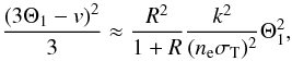 (21)where
 and ρb is the energy density of baryons. At
z > 105, when the
μ-type distortions are created, R2 ≪ 1 and
thermal conductivity contributes negligibly to the sound wave dissipation. The dominant
terms during the μ-type era are the second and the third (shear viscosity)
terms (Zaldarriaga & Harari 1995)
and ρb is the energy density of baryons. At
z > 105, when the
μ-type distortions are created, R2 ≪ 1 and
thermal conductivity contributes negligibly to the sound wave dissipation. The dominant
terms during the μ-type era are the second and the third (shear viscosity)
terms (Zaldarriaga & Harari 1995)
 (22)If
we ignore polarization, the factor of 16/15 in the above equation would
be replaced by 8/9. At redshifts z ≳ 2 × 10⁶
the distortions are exponentially suppressed due to the combined action of bremsstrahlung
and double Compton, which can create and destroy photons at low frequencies, and
comptonization, which redistributed the photons over the entire spectrum creating a
Bose-Einstein spectrum. The rate of energy injection in Eq. (20)therefore has to be multiplied by a suppression factor or blackbody
visibility,
(22)If
we ignore polarization, the factor of 16/15 in the above equation would
be replaced by 8/9. At redshifts z ≳ 2 × 10⁶
the distortions are exponentially suppressed due to the combined action of bremsstrahlung
and double Compton, which can create and destroy photons at low frequencies, and
comptonization, which redistributed the photons over the entire spectrum creating a
Bose-Einstein spectrum. The rate of energy injection in Eq. (20)therefore has to be multiplied by a suppression factor or blackbody
visibility,  ,
for z ≳ 105, giving the part of the energy injection which is
actually observed as μ-type distortion. An analytic solution for
was calculated by Sunyaev & Zeldovich
(1970c), who only considered bremsstrahlung. Their solution was later applied to
double Compton scattering by Danese & de Zotti
(1982) (accurate to 5−10%) and improved recently to sub-percent accuracy in Khatri & Sunyaev (2012). Numerical computation of
the spectral distortions is possible using numerical codes such as kyprix (Procopio & Burigana 2009) and
CosmoTherm9 (Chluba & Sunyaev 2012), the later code includes the energy
injection due to Silk damping and is able to calculate such small distortions at high
precision.
,
for z ≳ 105, giving the part of the energy injection which is
actually observed as μ-type distortion. An analytic solution for
was calculated by Sunyaev & Zeldovich
(1970c), who only considered bremsstrahlung. Their solution was later applied to
double Compton scattering by Danese & de Zotti
(1982) (accurate to 5−10%) and improved recently to sub-percent accuracy in Khatri & Sunyaev (2012). Numerical computation of
the spectral distortions is possible using numerical codes such as kyprix (Procopio & Burigana 2009) and
CosmoTherm9 (Chluba & Sunyaev 2012), the later code includes the energy
injection due to Silk damping and is able to calculate such small distortions at high
precision.
6. Conclusions
Mixing of blackbody spectra results in a photon distribution which is no longer a perfect blackbody but contains a y-type spectral distortion. The mixed spectrum has higher entropy than the average entropy of initial spectra as expected from an irreversible process which creates disorder. The energy which goes into the spectral distortion and the increase of entropy can be calculated very simply using statistical physics. The increase in entropy is, at first order in small distortions, independent of the shape of the distortion and can be calculated using the equilibrium thermodynamics formula for small addition of heat, dS = dQ/T. The part of the energy which sources distortions is only 1/3 of the total energy available in temperature perturbations (with respect to a blackbody at average initial temperature) and also results in increase of entropy. The remaining 2/3 of the energy in perturbations goes into increasing the average blackbody temperature of the photons and can be identified with entropy conserving part of the mixing process. We have proven explicitly in this paper that the comptonization of the initial spectrum with y-type distortion to the Bose-Einstein spectrum does not change this 2:1 division of the dissipated energy into a blackbody part and a distortion part. From an observational point of view, we are just interested in the value of the observable μ, and this 2:1 division of dissipated energy allows us to compute the value of μ in a straightforward way. μ-distortions are unique and very important because it is impossible to create them after z ≲ 105 and thus probe the physics of the early Universe unambiguously. y-type distortions on the other hand are created throughout the later history of the Universe, and it is difficult to separate the contributions from the different epochs.
We have an almost perfect blackbody in the Universe in the form of CMB. We apply our results to mixing of blackbodies in the observed CMB sky. As a result of this mixing, the spectrum observed by a telescope with finite beam size would have inevitable y-type distortions. This effect must be taken into account in experiments aiming to measure CMB spectrum at high precision. A very important application of physics of the mixing blackbodies is in the early Universe. Before recombination, the tightly coupled baryon-electron-photon plasma is excited by primordial perturbations in energy density, resulting in standing sound waves. The photons in different phases of the sound wave have a blackbody spectrum with different temperature. Photon diffusion and isotropization of the radiation field by Thomson scattering mixes these blackbodies on scales corresponding to diffusion length. These spectral distortions measure the primordial spectrum on very small scales (with the smallest scales completely inaccessible by any other means), at comoving wavenumbers 10 ≲ k ≲ 104 Mpc-1, and will thus provide a powerful new tool to constrain early Universe physics in the future. We have derived the energy release resulting from the damping of these sound waves, and the corresponding spectral distortions of the CMB, in a simple manner using the physics of mixing of blackbodies. These results and additional (but negligible) corrections were calculated recently using second order perturbation theory in Chluba et al. (2012b). The results, for the very important μ type distortions, coincidentally are close to the estimates used in literature until now, with the main difference being a correction factor of 3/4.
We discuss different processes which can lead to the mixing of blackbodies in the following sections.
In fact δn(x) is also invariant to change in the
reference temperature happening in the mixing of blackbodies,
![Mathematical equation: \hbox{$\delta n(x)=\delta n(x_{\rm {new}})+\mathcal{O}([\delta n/n]^2)$}](/articles/aa/full_html/2012/07/aa19590-12/aa19590-12-eq184.png) ,
where
xnew = ν/Tnew.
,
where
xnew = ν/Tnew.
Using 6ζ(3)/I3 ≈ 1.1106
and
π2/(3I2) ≈ 1.3684,
where ζ is the Riemann zeta function with
ζ(3) ≈ 1.20206, and  .
.
On very small scales the fluctuations are considerably smaller since these fluctuations were erased due to diffusion of photons before and during recombination (Silk damping).
Bold letters denote vectors, bold letters with hat denote unit vectors and normal letters denote magnitude of the vector.
We have ignored the gravitational potential/metric perturbations since they cannot create spectral distortions. They do cancel out explicitly in the second order Boltzmann equation (Chluba et al. 2012b). Gravitational potential/metric perturbations do contribute to the average CMB temperature but this effect is unobservable.
Our convention is same as that of (Ma & Bertschinger 1995; Dodelson 2003) but differs from that of Zaldarriaga & Harari (1995) by a factor of (− i)ℓ in the definition of multipole moments.
This does not introduce any error in the calculation of heating of the average CMB spectrum since we should average the sound wave over a whole oscillation.
References
- Bartolo, N., Matarrese, S., & Riotto, A. 2007 [arXiv:astro-ph/0703496] [Google Scholar]
- Bennett, C. L., Banday, A. J., Gorski, K. M., et al. 1996, ApJ, 464, L1 [NASA ADS] [CrossRef] [Google Scholar]
- Chluba, J., & Sunyaev, R. A. 2004, A&A, 424, 389 [NASA ADS] [CrossRef] [EDP Sciences] [Google Scholar]
- Chluba, J., & Sunyaev, R. A. 2006, A&A, 458, L29 [NASA ADS] [CrossRef] [EDP Sciences] [Google Scholar]
- Chluba, J., & Sunyaev, R. A. 2012, MNRAS, 419, 1294 [NASA ADS] [CrossRef] [Google Scholar]
- Chluba, J., Erickcek, A. L., & Ben-Dayan, I. 2012a, ApJ, submitted [arXiv:1203.2681] [Google Scholar]
- Chluba, J., Khatri, R., & Sunyaev, R. A. 2012b, MNRAS, submitted [arXiv:1202.0057] [Google Scholar]
- Daly, R. A. 1991, ApJ, 371, 14 [NASA ADS] [CrossRef] [Google Scholar]
- Danese, L., & de Zotti, G. 1982, A&A, 107, 39 [NASA ADS] [Google Scholar]
- Dent, J. B., Easson, D. A., & Tashiro, H. 2012 [arXiv:1202.6066] [Google Scholar]
- Dodelson, S. 2003, Modern cosmology (Amsterdam: Academic Press) [Google Scholar]
- Fixsen, D. J., & Mather, J. C. 2002, ApJ, 581, 817 [NASA ADS] [CrossRef] [Google Scholar]
- Fixsen, D. J., Cheng, E. S., Gales, J. M., et al. 1996, ApJ, 473, 576 [NASA ADS] [CrossRef] [Google Scholar]
- Ganc, J., & Komatsu, E. 2012 [arXiv:1204.4241] [Google Scholar]
- Hu, W., & Sugiyama, N. 1995, ApJ, 444, 489 [NASA ADS] [CrossRef] [Google Scholar]
- Hu, W., Scott, D., & Silk, J. 1994a, ApJ, 430, L5 [NASA ADS] [CrossRef] [Google Scholar]
- Hu, W., Scott, D., & Silk, J. 1994b, Phys. Rev. D, 49, 648 [NASA ADS] [CrossRef] [Google Scholar]
- Illarionov, A. F., & Sunyaev, R. A. 1975, SvA, 18, 691 [NASA ADS] [Google Scholar]
- Jarosik, N., Bennett, C. L., Dunkley, J., et al. 2011, ApJS, 192, 14 [NASA ADS] [CrossRef] [Google Scholar]
- Kaiser, N. 1983, MNRAS, 202, 1169 [NASA ADS] [Google Scholar]
- Khatri, R., & Sunyaev, R. A. 2012 [arxiv:1203.2601] [Google Scholar]
- Khatri, R., Sunyaev, R. A., & Chluba, J. 2012, A&A, 540, A124 [Google Scholar]
- Kogut, A., Fixsen, D. J., Chuss, D. T., et al. 2011, J. Cosmol. Astropart. Phys., 025 [Google Scholar]
- Komatsu, E., Smith, K. M., Dunkley, J., et al. 2011, ApJS, 192, 18 [NASA ADS] [CrossRef] [Google Scholar]
- Kompaneets, A. S. 1956, Zh. Eksp. Teor. Fiz., 31, 876 [Google Scholar]
- Landau, L. D., & Lifshitz, E. M. 1980, Statistical physics, Part. 1 (Oxford: Butterworth-Heinemann) [Google Scholar]
- Lifshitz, E. M. 1946, J. Phys. (USSR), 10, 116 [Google Scholar]
- Ma, C.-P., & Bertschinger, E. 1995, ApJ, 455, 7 [NASA ADS] [CrossRef] [Google Scholar]
- Pajer, E., & Zaldarriaga, M. 2012 [arXiv:1201.5375] [Google Scholar]
- Peebles, P. J. E., & Yu, J. T. 1970, ApJ, 162, 815 [NASA ADS] [CrossRef] [Google Scholar]
- Pitrou, C. 2009, Class. Quant. Grav., 26, 065006 [NASA ADS] [CrossRef] [Google Scholar]
- Procopio, P., & Burigana, C. 2009, A&A, 507, 1243 [NASA ADS] [CrossRef] [EDP Sciences] [Google Scholar]
- Rubiño-Martín, J. A., Chluba, J., & Sunyaev, R. A. 2008, A&A, 485, 377 [NASA ADS] [CrossRef] [EDP Sciences] [Google Scholar]
- Silk, J. 1968, ApJ, 151, 459 [NASA ADS] [CrossRef] [Google Scholar]
- Sunyaev, R. A., & Zeldovich, Y. B. 1970a, Ap&SS, 9, 368 [NASA ADS] [CrossRef] [Google Scholar]
- Sunyaev, R. A., & Zeldovich, Y. B. 1970b, Ap&SS, 7, 3 [NASA ADS] [Google Scholar]
- Sunyaev, R. A., & Zeldovich, Y. B. 1970c, Ap&SS, 7, 20 [Google Scholar]
- Weinberg, S. 1971, ApJ, 168, 175 [Google Scholar]
- Zaldarriaga, M., & Harari, D. D. 1995, Phys. Rev. D, 52, 3276 [NASA ADS] [CrossRef] [Google Scholar]
- Zeldovich, Y. B., & Sunyaev, R. A. 1969, Ap&SS, 4, 301 [NASA ADS] [CrossRef] [Google Scholar]
- Zeldovich, Y. B., Illarionov, A. F., & Sunyaev, R. A. 1972, Sov. J. Exper. Theor. Phys., 35, 643 [Google Scholar]
All Figures
|
Fig. 1 Average of blackbodies of temperature T + ΔT and T − ΔT creates a new spectrum marked “Average(Y)” which is different from blackbody spectrum marked with temperature T. The average spectrum is just the usual y-type distortion with respect to a new blackbody at temperature T [1 + (ΔT/T)2] , with the two crossing at x = 3.83. At redshifts z ≳ 105 the average spectrum will comptonize to Bose-Einstein spectrum marked μ above. All three spectra, T [1 + (ΔT/T)2] , Average (Y), and μ, have the same number density of photons. Average/y-type spectrum and Bose-Einstein/μ-type spectrum also have the same energy density which is greater than the energy density in the blackbody spectrum with temperature T [1 + (ΔT/T)2] by 1/3 of the initial energy density excess over that of blackbody with temperature T. We have used linear order formulae to calculate the y and μ distortions in the figure but used a large value of ΔT/T to make differences between different curves visible. |
| In the text | |
|
Fig. 2 Same as Fig. 1 but effective temperature Teff(ν) defined by n(ν) = 1/(eν/Teff(ν) − 1) is plotted. We have used linear order formulae to calculate the y and μ distortions in the figure but used a large value of ΔT/T = 0.4 to make differences between different curves visible. Average temperature T = 2.725 K. For Bose-Einstein spectrum we thus have, at linear order, Teff(x) = TBE − Tμ/x. For a general distortion δn/n (including y-type ) we have Teff(x) = T + T[(1−e−x)/x]δn/n. |
| In the text | |
|
Fig. 3 Cartoon picture of mixing of blackbodies: photons from different phases of sound wave mix and create spectral distortion/entropy. |
| In the text | |
Current usage metrics show cumulative count of Article Views (full-text article views including HTML views, PDF and ePub downloads, according to the available data) and Abstracts Views on Vision4Press platform.
Data correspond to usage on the plateform after 2015. The current usage metrics is available 48-96 hours after online publication and is updated daily on week days.
Initial download of the metrics may take a while.