| Issue |
A&A
Volume 541, May 2012
|
|
|---|---|---|
| Article Number | A113 | |
| Number of page(s) | 4 | |
| Section | Stellar structure and evolution | |
| DOI | https://doi.org/10.1051/0004-6361/201218881 | |
| Published online | 10 May 2012 | |
Research Note
Gravity-darkening exponents and apsidal-motion constants for pre-main-sequence models⋆
Instituto de Astrofísica de Andalucía, CSIC, Apartado 3004, 18080 Granada, Spain
e-mail: This email address is being protected from spambots. You need JavaScript enabled to view it.
Received: 24 January 2012
Accepted: 28 March 2012
Abstract
Context. The apsidal-motion constants kj and the moment of inertia are often used to study the apsidal-motion and tidal evolution of double-lined eclipsing binaries and planetary systems. On the other hand, the computation of the theoretical light curves of eclipsing binaries, planetary transits, and single rapidly rotating stars requires the knowledge of how the flux is distributed over the distorted stellar surfaces which can derived from the gravity-darkening exponent. Such parameters are available for several masses and chemical compositions covering the main sequence and giant branch. However, for early phases (pre-main sequence, hereafter PMS) the calculations are scarce or even lacking.
Aims. We present the calculations of the apsidal-motion constants, the fractional radius of gyration, and the gravity-darkening exponents for an extensive grid of PMS.
Methods. The code used to generate the PMS models is essentially the same as that described by us in 2004. The apsidal-motion constants, the moment of inertia and the potential energy were computed using a fourth order Runge-Kutta method. The gravity-darkening exponents were computed using a method previously developed by us.
Results. The apsidal-motion constants, the moment of inertia, the potential energy, and the gravity-darkening exponents are made available for each point on every evolutionary track for PMS models covering the mass range 0.05–30 M⊙. Our calculations are made available for three chemical compositions (X,Z) = (0.757, 0.001), (0.70, 0.02), (0.64, 0.04).
Key words: binaries: eclipsing / stars: evolution / stars: pre-main sequence / stars: interiors / stars: rotation
Tables 1abc–20abc are only available at the CDS via anonymous ftp to cdsarc.u-strasbg.fr (130.79.128.5) or via http://cdsarc.u-strasbg.fr/viz-bin/qcat?J/A+A/541/A113 Additional data are available upon request.
© ESO, 2012
1. Introduction
The distortions in the shape of binary stars due to proximity effects cause a slow rotation of the line of the apses, known as apsidal-motion, that provides a robust tool for searching into the interior of the stars. These distortions can be calculated as a function of the internal structure of the stars (Kopal 1978). An accurate measurement of this phenomenon can be obtained by monitoring the primary and secondary minima of eclipsing binaries. The resulting empirical apsidal-motion rates can be compared with the theoretical ones, derived from evolutionary stellar models. For an update of the comparison theory-observations, we refer to Claret & Giménez (2010) and, for relativistic systems, sto Claret (1997) and more recently Wolf et al. (2010).
Tidal evolution can also be used to investigate the interior of the stars. The available approximations to the differential equations that govern the orbital elements depend on the moment of inertia of each star and in some formalisms, also the apsidal-motion constants (see for example, Hut 1981; Eggleton & Kiseleva-Eggleton 2002). One of the first calculations of a stellar moment of inertia was carried out by Motz (1952). However, the adopted models at that time were too simple. The first attempt to produce a systematic calculation of the fractional radius of gyration was that of Claret & Giménez (1998), who tabulated the fractional radius of gyration for a grid of hydrogen-burning stars for use in stellar dynamics. Later, in Claret & Giménez (1991), the same authors investigated the influence of core overshooting and mass loss on the internal structure constants.
In relation still to stellar distortions, the computation of the theoretical light curves of eclipsing binaries, planetary transits, and single rapidly rotating stars requires the knowledge of how the flux is distributed over the distorted stellar surfaces. There are two important historical papers that provide the values of the gravity-darkening exponents (GDE) β1: that of von Zeipel (1924), which treats stars with radiative envelopes (β1 = 1.0), and that of Lucy (1967), who used convective envelopes, which are appropriate for late-type stars, to derive an average of β1 = 0.32. These values were used over several decades until the paper of Claret (1998), who introduced a numerical method based on the triangles strategy of Kippenhahn et al. (1967, which provides values of the gravity-darkening exponents as a function of age, mass, and chemical composition. A smooth transition in the values of β1 is achieved between the convective/radiative transport of energy.
All the aforementioned parameters are presently available for several masses and chemical compositions covering evolutionary phases such as the main sequence (MS) and red giant branch but for early phases the calculations are very scarce or even lacking. In the present paper, we present the calculations of the apsidal-motion constants, the fractional radius of gyration, and the gravity-darkening exponents for an extensive grid of PMS. These calculations can be used to investigate the apsidal-motion of double-lined eclipsing binaries, the tidal evolution, and the brightness distribution of very young stars.
2. The stellar models
The code used to generate the PMS models is essentially the same as that described in Claret (2004). For completeness, we give some of its main characteristics describing PMS evolution. We adopt the equation of state OPAL (Rogers et al. 1996). The code uses the opacity tables provided by Iglesias & Rogers (1996), which are completed by the calculations by Ferguson et al. (2005) for lower temperatures. We adopt X = 0.70 and Z = 0.02, which is representative of a typical chemical composition. Two additional compositions are available of (X,Z) = (0.757, 0.001) and (0.64, 0.04).
Convection was treated by using the mixing-length theory (αMLT = 1.5) and we adopt the Schwarzschild criterion to delineate the convective boundaries. To get more accurate computations we decreased the triangle size used to define an envelope in Herzsprung-Russel (HR) diagram to Δlog Teff = 0.001 and Δlog L = 0.004. This is particularly important to determinate the depth of the convective envelope. The calculations cover the mass range 0.05–30 M⊙ (Table 1). All models were computed using our stellar evolution code (Claret 2004), except those with masses 0.05, 0.1, 0.2, and 0.4 M⊙ for which we used the MESA code (Paxton et al. 2011). Figure 1 shows the HR diagram for the PMS models with (X,Z, αMLT) = (0.70, 0.02, 1.5).
List of available models.
3. Gravity-darkening exponents, apsidal-motion constants, radius of gyration and potential energy
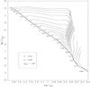 |
Fig. 1 Evolutionary tracks for PMS models. Attached numbers denote the masses of the model in solar units. |
We introduce the equations and numerical methods necessary to calculate the gravity-darkening exponents, the radius of gyration, the potential energy, and the internal structure constants. The gravity-darkening exponent is an important parameter that is often used in the analysis of the light curves of eclipsing binaries and the modelling of rapidly rotating stars. For stars in strict radiative equilibrium (pseudo-barotrope), von Zeipel (1924) showed that the variation in the brightness over the surface is proportional to the effective gravity: 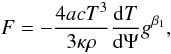 (1)or
(1)or  (2)where β1 = 1.0, g is the local gravity, Ψ is the total potential, and the remaining variables have their usual meaning in studies of stellar structure. Lucy (1967) computed values of β1 for convective envelopes, finding an average value of 0.32. As mentioned in the introduction, we have introduced a numerical method to compute β1, that allows us to calculate the gravity-darkening exponents as a function of age, mass, chemical composition, etc. Such a method provides a set of β1 that supersedes the old values of 0.32 and 1.0 for convective and radiative envelopes respectively and a smooth transition is achieved between both energy transport mechanisms. The aforementioned smooth transition zone was confirmed by the observations of Che et al. (2011) for very rapid rotators.
The numerical method is based on the triangles strategy (Claret 1998). Given that the external boundary conditions are unchanged during the evolution, the integrations in the outer layers will be the same, provided that the corresponding triangles in the HR diagram are small. By generalizing to several points, we can then simulate distorted configurations with different effective temperature distributions over the surface. The numerical differentiation of these envelopes allows us, finally, to obtain β1. A variation in this method was presented in Claret (2012), where the GDE were computed as a function of the optical depth. In that paper, we showed that the classical von Zeipel’s theorem (β1 = 1.0) is not strictly valid in the upper layers of hot rotating stars.
We derive the theoretical apsidal-motion constants kj by integrating the differential equations of Radau 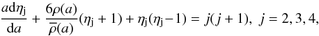 (3)where
  (4)and a is the mean radius of the configuration, ϵj is the deviation from sphericity, ρ(a) is the mass density at the distance a from the centre, and
  is the mean mass density within a sphere of radius a. The kj are computed using
 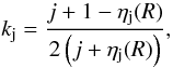 (5)where R refers the values of ηj at the stellar surface.
The fractional radius of gyration β is obtained for each stellar configurations using  (6)and the potential energy
  (7)where the form-factors β and α describe the moment of inertia and the potential energy, respectively. Equations (3), (6), and (7) were integrated using a fourth order Runge-Kutta method and the values of kj, β, and α were finally derived.
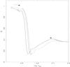 |
Fig. 2 The gravity-darkening exponent evolution. The continuous line represents a 2 M⊙ during the PMS phase, while the dashed line denotes the same model after the PMS stage. The two arrows indicate the direction of the evolution in both cases. |
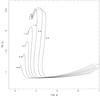 |
Fig. 3 The apsidal-motion constant log k2 as a function of mass and log g for some selected PMS models. The attached numbers indicate the model mass in solar units. |
A contracting model with 2 M⊙ is very useful to illustrate the evolution of β1 (Fig. 2). The continuous line represents the PMS-ZAMS phase and the dashed one denotes the post ZAMS models. The arrows indicate the time evolution direction. In the first stages of PMS, the depth of the convective envelope is large and decreases progressively as the star approaches the ZAMS. The corresponding β1 is almost constant in this range. Outside this interval, this value increases, reaching a local maximum around log Teff = 3.70. This behaviour is due to the onset of the convection: the convection is present even in thin layers. For effective temperatures lower than 5000 K, there is a decrease in the optical depth where convection appears. The hydrogen recombination is responsible for this and the efficiency of the convection is higher. For higher effective temperatures, convection loses importance and the corresponding β1 decreases until a local minimum at log Teff ≈ 3.84 (that value depends on the envelope input physics). In addition, the von Zeipel value of β1 is progressively restored towards the ZAMS point.
During the PMS, β1 is systematically larger than the computed ones for later phases of log Teff < 3.84. Although the PMS and post-ZAMS models show similar effective temperatures, the respective physical conditions in the envelopes are different. When the depth of the convective envelopes are of the same order, β1 converges to similar values. This can be seen in particular at the beginning of the PMS or for models near the ZAMS.
Our codes which are designed to compute the GDE, do not include ingredients such as the evolution of the chemical abundance distribution caused by gravitational settling, chemical/thermal diffusion of the elements, or a more specific equation of state for very compact objects and therefore, for consistency, we do not calculate the gravity-darkening exponents for very low mass stars. These objects, owing to their peculiar characteristics, will be studied in a separate paper.
Figure 3 shows the evolution of log k2 as a function of log g for some selected PMS sequences. The masses (in solar units) are indicated in the figure. Two interesting features can be seen in Fig. 3. The first one is related to the first stages of the PMS tracks: the models have similar mass distributions which correspond to configurations with an effective polytropic index 1.5–2.0.
As the models evolve, they become more centrally condensed and, consequently, the apsidal-motion constant decreases. The second point refers to the double maxima in log k2, which appears for models with initial masses higher than 1.2 M⊙. These changes in the internal structure of the models when they are close to the ZAMS are due to the reduction in the original C12 through the nuclear reactions C12(p, γ)N13(β + , ν)C13(p, γ)N14. The models have a nuclear energy source, though the gravitational and thermal energies also contribute. The mass concentration either reduces or increases depending on the predominant source of energy. A similar characteristic is also detected in later evolutionary phases (for m > 1.2 M⊙) and is due to a change in the dominant nuclear source of energy from the proton-proton chain to CNO cycle.
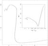 |
Fig. 4 Comparison between apsidal-motion constants log k2: with our stellar evolutionary code (continuous line) and that computed by using MESA (dashed line). The figure in the upper right corner shows a comparison of the corresponding HR diagram for the same models. The characteristics of the models are 3 M⊙, (X,Z, αMLT) = (0.70, 0.02, 1.5). |
Figure 4 compares the log k2 for a 3 M⊙ model computed using our stellar evolution code (Claret 2004, continuous line) with the evolution of log k2 computed with the MESA code (version 3290) recently developed by Paxton et al. (2011) denoted
by the dashed line. The agreement between the two calculations is very good in all phases of the PMS evolution. We also found very good agreement for later phases such as the MS or red giant branch. The figure at the upper right corner of Fig. 4 shows the corresponding HR diagram for the same models. The agreement can be considered to be good; the maximum differences in Teff are of the order of 1–3% in the either early stages or near ZAMS.
All calculations presented here for α and β have been performed for spherical configurations. However, in the case of elliptical symmetry and an ellipsoidal mass distribution the corresponding α and β can also be computed by writing them in terms of both the spherical structure and of a correction factor that depends on the geometry of the perturbation. We return to this specific subject in future investigations.
Finally, we note that the PMS tables contain 11 columns corresponding to the age (in years), the mass (solar units), log L (in solar units), log Teff, log g(cgs), log k2, log k3, log k4, α, β, and β1.
Acknowledgments
B. Paxton and A. Dotter are particularly acknowledged for their help in the implementating MESA. The Spanish MEC (AYA2009-10394, AYA2009-14000-C03-01) is gratefully acknowledged for its support during the development of this work. This research has made use of the SIMBAD database, operated at the CDS, Strasbourg, France, and of NASA’s Astrophysics Data System Abstract Service.
References
- Che, X., Monnier, J. D., Zhao, M., et al. 2011, ApJ, 732, 68 [NASA ADS] [CrossRef] [Google Scholar]
- Claret, A. 1997, A&A, 327, 11 [NASA ADS] [Google Scholar]
- Claret, A. 1998, A&AS, 131, 395 [NASA ADS] [CrossRef] [EDP Sciences] [Google Scholar]
- Claret, A. 2004, A&A, 424, 919 [NASA ADS] [CrossRef] [EDP Sciences] [Google Scholar]
- Claret, A. 2012, A&A, 538, A3 [NASA ADS] [CrossRef] [EDP Sciences] [Google Scholar]
- Claret, A., & Giménez, A. 1989, A&AS, 81, 37 [NASA ADS] [Google Scholar]
- Claret, A., & Giménez, A. 1991, A&A, 244, 319 [NASA ADS] [Google Scholar]
- Claret, A., & Giménez, A. 2010, A&A, 519, A57 [NASA ADS] [CrossRef] [EDP Sciences] [Google Scholar]
- Eggleton, P. P., & Kiseleva-Eggleton, L. 2002, ApJ, 575, 461 [NASA ADS] [CrossRef] [Google Scholar]
- Ferguson, J. W., Alexander, D. R., Allard, F., et al. 2005, ApJ, 623, 585 [NASA ADS] [CrossRef] [Google Scholar]
- Hut, P. 1981, A&A, 99, 126 [NASA ADS] [Google Scholar]
- Iglesias, C. A., & Rogers, F. J. 1996, ApJ, 464, 943 [NASA ADS] [CrossRef] [Google Scholar]
- Kippenhahn, R., Weigert, A., & Hofmeister, E. 1967, in Comp. Phys. (New York: Academic Press), 7, 129 [Google Scholar]
- Kopal, Z. 1978, Dynamics of Close Binary Systems (Dordrecht Holland: Reidel) [Google Scholar]
- Lucy, L. B. 1967, Z. Astrophys., 65, 89 [Google Scholar]
- Motz, L. 1952, ApJ, 115, 562 [Google Scholar]
- Paxton, B., Bildsten, L., Dotter, A., et al. 2011, ApJS, 192, 3 [Google Scholar]
- Rogers, F. J., Iglesias, C. A., & Swenson, F. J. 1996, ApJ, 456, 902 [NASA ADS] [CrossRef] [Google Scholar]
- von Zeipel, H. 1924, MNRAS, 84, 665 [NASA ADS] [CrossRef] [Google Scholar]
- Wolf, M., Claret, A., Kotkova, H., et al. 2010, A&A, 509, A18 [NASA ADS] [CrossRef] [EDP Sciences] [Google Scholar]
All Tables
All Figures
|
Fig. 1 Evolutionary tracks for PMS models. Attached numbers denote the masses of the model in solar units. |
| In the text | |
|
Fig. 2 The gravity-darkening exponent evolution. The continuous line represents a 2 M⊙ during the PMS phase, while the dashed line denotes the same model after the PMS stage. The two arrows indicate the direction of the evolution in both cases. |
| In the text | |
|
Fig. 3 The apsidal-motion constant log k2 as a function of mass and log g for some selected PMS models. The attached numbers indicate the model mass in solar units. |
| In the text | |
|
Fig. 4 Comparison between apsidal-motion constants log k2: with our stellar evolutionary code (continuous line) and that computed by using MESA (dashed line). The figure in the upper right corner shows a comparison of the corresponding HR diagram for the same models. The characteristics of the models are 3 M⊙, (X,Z, αMLT) = (0.70, 0.02, 1.5). |
| In the text | |
Current usage metrics show cumulative count of Article Views (full-text article views including HTML views, PDF and ePub downloads, according to the available data) and Abstracts Views on Vision4Press platform.
Data correspond to usage on the plateform after 2015. The current usage metrics is available 48-96 hours after online publication and is updated daily on week days.
Initial download of the metrics may take a while.