| Issue |
A&A
Volume 538, February 2012
|
|
|---|---|---|
| Article Number | A65 | |
| Number of page(s) | 15 | |
| Section | Astronomical instrumentation | |
| DOI | https://doi.org/10.1051/0004-6361/201015785 | |
| Published online | 03 February 2012 | |
Bayesian analysis of polarization measurements
Pontificia Universidad Católica de Chile, Departamento de Astronomía y
Astrofísica,
Vicuña Mackenna 4860, Macul
690-4411
Santiago
Chile
e-mail: This email address is being protected from spambots. You need JavaScript enabled to view it.
Received:
19
September
2010
Accepted:
25
October
2011
Abstract
Context. A detailed and formal account of polarization measurements using Bayesian analysis is given based on the assumption of gaussian error for the Stokes parameters. This analysis is crucial for the measurement of the polarization degree and angle at low and high signal-to-noise. The treatment serves as a framework for customized analysis of data based on a particular prior suited to the experiment.
Aims. The aim is to provide a rigorous and self-consistent Bayesian treatment of polarization measurements and their statistical error focused on the case of a single measurement.
Methods. Bayes Theorem is used to derive a variety of posterior distributions for polarization measurements.
Results. A framework that may be used to construct accurate polarization point estimates and confidence intervals based on Bayesian ideas is given. The results may be customized for a prior and loss function chosen for a particular experiment.
Key words: polarization / methods: data analysis
© ESO, 2012
1. Introduction
Measuring polarization presents several challenges. The most important are that a naive calculation of small polarization seems to be biased towards higher values (Serkowski 1958), the error bars of the measured polarization are non-symmetric below a threshold signal-to-noise (Simmons & Stewart 1985), and the angular distribution is non-gaussian (Naghizadeh-Khouei & Clarke 1993). Given measured values of the Stokes parameters, what are the best estimates for the true values of the polarization degree and angle and how should error bars be assigned?
The polarization state of quasi-monochromatic light may be stated in terms of
I0, Q0,
U0, and V0 Stokes parameters which
are defined as certain averages of the electric field along a pair of orthogonal axes
perpendicular to the direction of the light’s propagation (see, e.g., del Toro Iniesta (2003) or Landi
Degl’Innocenti (2002) for more information). I0 is the
intensity, Q0 and U0 are related to
linear polarization, and V0 is circular polarization. The Stokes
parameters are subject to two conditions: 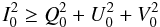 (1)and
 (2)If incoming light is
totally polarized, then the equality holds in Eq. (1), otherwise it is partially polarized or unpolarized. To keep the equations of
manageable size, the rest of this paper makes the assumption that circular polarization is
negligible (i.e., V0 = 0). It should be straight-forward to
generalize the results to include a non-zero V0. This
restriction is not very severe because circular polarization is small compared to linear
polarization for many astrophysical sources. It will also be taken that the Stokes
parameters are constant during the course of a single observation.
(2)If incoming light is
totally polarized, then the equality holds in Eq. (1), otherwise it is partially polarized or unpolarized. To keep the equations of
manageable size, the rest of this paper makes the assumption that circular polarization is
negligible (i.e., V0 = 0). It should be straight-forward to
generalize the results to include a non-zero V0. This
restriction is not very severe because circular polarization is small compared to linear
polarization for many astrophysical sources. It will also be taken that the Stokes
parameters are constant during the course of a single observation.
Stokes parameters are calculated from intensities that follow a Poisson distribution governed by photon counts. Clarke et al. (1983) and Maronna et al. (1992) have investigated this to make optimal estimates of them from repeated measurements. In general, however, a full Poisson treatment is computationally difficult when large intensities are involved. To avoid concerns about Poisson statistics, it is assumed that all intensities used to calculate Q and U (and also I) are large enough to be treated as having gaussian distributions.
The specifics regarding the calculation of I, Q,
U and their errors ( ,
,
 ,
,
 ) depend on the
experimental design (Keller 2002). For example, if
one is using a dual-beam polarimeter with a half-wave-plate, Patat & Romaniello (2006) present an optimal set of equations for
calculating the Stokes parameters from the intensities of the ordinary and extraordinary
beams at different waveplate angles. Since the assumption that these intensities are large
enough to be approximated by a Gaussian is being made, this implies that one may use the
usual Gaussian error propagation formula for ,
, and
based on the errors for
the individual intensities (square root of the counts) that went into their calculation.
Regardless how I, Q, and U are actually
calculated, they may be treated as logically separate (e.g., one could imagine one
instrument measuring intensity with error in conjunction with
completely separate instruments measuring Q and U with
errors and
, respectively). Hereon,
the error on the measured total intensity, , is treated as being
independent of and
.
) depend on the
experimental design (Keller 2002). For example, if
one is using a dual-beam polarimeter with a half-wave-plate, Patat & Romaniello (2006) present an optimal set of equations for
calculating the Stokes parameters from the intensities of the ordinary and extraordinary
beams at different waveplate angles. Since the assumption that these intensities are large
enough to be approximated by a Gaussian is being made, this implies that one may use the
usual Gaussian error propagation formula for ,
, and
based on the errors for
the individual intensities (square root of the counts) that went into their calculation.
Regardless how I, Q, and U are actually
calculated, they may be treated as logically separate (e.g., one could imagine one
instrument measuring intensity with error in conjunction with
completely separate instruments measuring Q and U with
errors and
, respectively). Hereon,
the error on the measured total intensity, , is treated as being
independent of and
.
Most of the polarization error literature makes the further assumption that the measured
Stokes parameters are normally distributed about their true values,
Q0 and U0, with standard deviation
and
. It is also usually
assumed that the Q and U distributions are characterized
by equal dispersion. Unfortunately,  is not generally
satisfied for arbitrary datasets. This assumption is a pragmatic one to avoid ellipsoidal
distributions which would complicate the analysis. Careful design of the experiment can make
it such that
is not generally
satisfied for arbitrary datasets. This assumption is a pragmatic one to avoid ellipsoidal
distributions which would complicate the analysis. Careful design of the experiment can make
it such that  . Extension of the
results to allow for unequal variance is reserved for future work. It is now assumed that
and
are equal and called Σ.
The quantity only tangentially enters
the analysis, leaving Σ as the lone important error quantity. In practice, Σ could be set
equal to the average of and
or the maximum value if
one is more conservative.
. Extension of the
results to allow for unequal variance is reserved for future work. It is now assumed that
and
are equal and called Σ.
The quantity only tangentially enters
the analysis, leaving Σ as the lone important error quantity. In practice, Σ could be set
equal to the average of and
or the maximum value if
one is more conservative.
The units on I, Q, U and
,
,
are energy per time.
Shortly, new variables will be defined that are unitless. They will be best interpreted as
percentages or ratios and the issue of units vanishes.
2. Theoretical background
In this section, the various distributions that will be needed are derived. The distributions will be presented in several different coordinate systems because this is intended to serve as a reference and because it is exceedingly easy to miss factors introduced by the Jacobian.
2.1. The sampling distribution
2.1.1. Variable introductions and large intensity limit
The fundamental assumption of this paper is that the measurement of the (unnormalized)
Stokes parameters, Q and U, which are assumed to be
uncorrelated, is described by a two-dimensional gaussian with equal standard deviation,
Σ, in both directions. This distribution, FC, is
 (3)(Most of the work for
this paper will be done in polar coordinates. A C-subscript will be
used for distributions in Cartesian coordinates.) The value of Σ is a positive constant
assumed to be known precisely and, in practice, is estimated from the data. The
parameters, Q0 and U0, must be
elements of a disk of radius I0 centered on the origin in
the Q0-U0 plane. The range of
both Q and U is (−∞,∞) due to
measurement error although the probability of measuring a value outside a disk of radius
I0 diminishes rapidly even for values of
Q0 and U0 near the rim.
Equation (3) is normalized
(
(3)(Most of the work for
this paper will be done in polar coordinates. A C-subscript will be
used for distributions in Cartesian coordinates.) The value of Σ is a positive constant
assumed to be known precisely and, in practice, is estimated from the data. The
parameters, Q0 and U0, must be
elements of a disk of radius I0 centered on the origin in
the Q0-U0 plane. The range of
both Q and U is (−∞,∞) due to
measurement error although the probability of measuring a value outside a disk of radius
I0 diminishes rapidly even for values of
Q0 and U0 near the rim.
Equation (3) is normalized
( ).
).
It is often helpful to work in normalized Stokes parameters. Define new variables
q ≡ Q/I0,
u ≡ U/I0,
q0 ≡ Q0/I0,
u0 ≡ U0/I0,
and σ ≡ Σ/I0. The scaled
error, σ, is an admixture between the intensity and the mean
Q-U error. It or its inverse,
1/σ
=I0/Σ, may be regarded as a measure of
data quality (cf.  ,
,
 , and
, and
 ). Small
σ (large 1/σ) implies good data.
The values for q0 and u0 are
restricted to a unit disk centered on the origin. The new probability density,
fC, after the change of coordinates is
). Small
σ (large 1/σ) implies good data.
The values for q0 and u0 are
restricted to a unit disk centered on the origin. The new probability density,
fC, after the change of coordinates is  (4)This equation is also
normalized (
(4)This equation is also
normalized ( ).
).
The normalized Stokes parameters q and u present a minor problem. How can they be calculated if I0 is an unknown quantity? It might be thought that the definition of q and u should use the measured intensity, I, instead of the true intensity, I0. If that alternative definition is used, however, the differentials of q and u are more complicated than just dq = dQ/I0 and du = dU/I0. This makes a change of variables for the distribution difficult. It is better to keep the first definition and require that I0 ≈ I. This occurs when the total number of counts that went into the measurement of I is large, which also implies ΣI ≪ I.
Another helpful set of variables are “signal-to-noise” ratios. They are defined by
 ,
,
 ,
,
 , and
, and
 . In
these barred variables, the new distribution,
. In
these barred variables, the new distribution,  , is
, is
 (5)This time, the Jacobian
causes the 1/σ2 leftover after the change
of variables to disappear. This is normalized as well
(
(5)This time, the Jacobian
causes the 1/σ2 leftover after the change
of variables to disappear. This is normalized as well
( ); but, in this case,
 and
and
 are restricted
to a disk of radius 1/σ.
are restricted
to a disk of radius 1/σ.
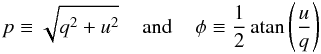
2.1.2. Transformation to polar coordinates
The true polarization degree, p0, and true angle on the
sky,  , may be defined in
terms of the true (i.e., perfectly known) q0 and
u0 Stokes parameters by
, may be defined in
terms of the true (i.e., perfectly known) q0 and
u0 Stokes parameters by  (6)The true angle on the
sky is related to the true angle in the
q0 − u0 plane by the relation
(6)The true angle on the
sky is related to the true angle in the
q0 − u0 plane by the relation
 . Similarly,
 (7)and
θ ≡ 2φ. The range of p is
[0,∞) and the range of p0 is
[0,1] . Define
(7)and
θ ≡ 2φ. The range of p is
[0,∞) and the range of p0 is
[0,1] . Define  and
and
 . It
is important to notice that the range of
. It
is important to notice that the range of  is now
[0,1/σ] or
[0,I0/Σ] because
in the Bayesian analysis, this will be the range of integration. The polarization angle
defines the plane of vibration of the electric field on the sky. By convention, it is
usually defined such that 0° corresponds to North and increases eastward such
that East is φ = 90°.
is now
[0,1/σ] or
[0,I0/Σ] because
in the Bayesian analysis, this will be the range of integration. The polarization angle
defines the plane of vibration of the electric field on the sky. By convention, it is
usually defined such that 0° corresponds to North and increases eastward such
that East is φ = 90°.
Equation (4) may be converted to polar
coordinates by inverting Eqs. (6)
and (7). Using θ
instead of φ, this yields
q = pcosθ and
u = psinθ and corresponding
equations for the zero-subscripted true values. The normalized probability density
distribution in polar coordinates (p,θ) is 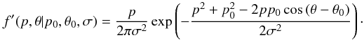 (8)A prime is used as part
of the function’s name to serve as a warning that the angle in the
q − u plane, θ, is being used as
the angular variable. The factor of p in front enters because
dq du = p dp dθ
(i.e., due to the Jacobian of the transformation). Some authors choose to leave the
factor of p off of the p, θ-distribution and insert it
manually when needed. Probability distributions transform as a scalar density under
coordinate transformations so they should “pick-up” the Jacobian factor. Caution is
needed when reading the literature.
(8)A prime is used as part
of the function’s name to serve as a warning that the angle in the
q − u plane, θ, is being used as
the angular variable. The factor of p in front enters because
dq du = p dp dθ
(i.e., due to the Jacobian of the transformation). Some authors choose to leave the
factor of p off of the p, θ-distribution and insert it
manually when needed. Probability distributions transform as a scalar density under
coordinate transformations so they should “pick-up” the Jacobian factor. Caution is
needed when reading the literature.
The distribution in terms of the sky angle is 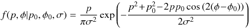 (9)and
in barred variables,
(9)and
in barred variables, 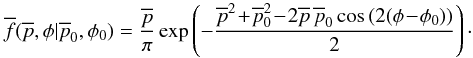 (10)The
 distribution is normalized
under the support
[0,∞) × (−π/2,π/2]
(i.e.,
distribution is normalized
under the support
[0,∞) × (−π/2,π/2]
(i.e.,  ). The
origin has infinitesimal measure so usually it does not contribute finitely to an
integral. In later sections, integration over delta functions (aka delta distributions)
centered at the origin will occur. This requires some formality in the polar coordinate
definition. The parameter space technically has
(p = 0,φ) identified for all φ as
the origin and (p,φ) is identified with
(p,φ = φ + nπ) for all
p > 0 and any integer n. The
resulting quotient space has
). The
origin has infinitesimal measure so usually it does not contribute finitely to an
integral. In later sections, integration over delta functions (aka delta distributions)
centered at the origin will occur. This requires some formality in the polar coordinate
definition. The parameter space technically has
(p = 0,φ) identified for all φ as
the origin and (p,φ) is identified with
(p,φ = φ + nπ) for all
p > 0 and any integer n. The
resulting quotient space has ![Mathematical equation: \hbox{$[0,\infty) \times{} (-\frac{\pi}{2},\frac{\pi}{2}]$}](/articles/aa/full_html/2012/02/aa15785-10/aa15785-10-eq94.png) as a fundamental cell.
Functions on this space are periodic in φ and they must satisfy
as a fundamental cell.
Functions on this space are periodic in φ and they must satisfy
 .
Here, “mod” is the modulus operator. The π/2
operations perform shifts needed because the angles are defined as
.
Here, “mod” is the modulus operator. The π/2
operations perform shifts needed because the angles are defined as
![Mathematical equation: \hbox{$(-\frac{\pi}{2},\frac{\pi}{2}]$}](/articles/aa/full_html/2012/02/aa15785-10/aa15785-10-eq97.png) instead of
[0,π). This formality is sometimes important in calculations, like
median estimates of φ0, where it is natural to have the
range of integration extend outside of the domain.
instead of
[0,π). This formality is sometimes important in calculations, like
median estimates of φ0, where it is natural to have the
range of integration extend outside of the domain.
 |
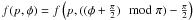
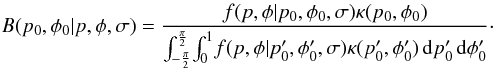
Fig. 1 Contour plots of |
Some intuition is gained by examining the distribution in Eq. (10) for differing values of
p0/σ. Figures 1a–c show the distributions for
 and
p0/σ = 0.0, 0.5 and
2.0, respectively. Choosing a different value of , for a given value
of p0/σ, only translates
the distribution in the φ-direction and does not change its shape;
therefore, all plots simply use . When
p0/σ = 0 the angular
distribution is flat and much of the probability is concentrated in a band around
p/σ = 1. As
p0/σ increases, an
oval-shaped “probability bubble” forms. This shape persists even at large values. The
probability under the distribution to the left and right of the maximum is asymmetric,
with more to the left. As
p0/σ continues to
increase, the probability on each side of the maximum approaches 0.5. This is true even
though the oval shape stays present.
and
p0/σ = 0.0, 0.5 and
2.0, respectively. Choosing a different value of , for a given value
of p0/σ, only translates
the distribution in the φ-direction and does not change its shape;
therefore, all plots simply use . When
p0/σ = 0 the angular
distribution is flat and much of the probability is concentrated in a band around
p/σ = 1. As
p0/σ increases, an
oval-shaped “probability bubble” forms. This shape persists even at large values. The
probability under the distribution to the left and right of the maximum is asymmetric,
with more to the left. As
p0/σ continues to
increase, the probability on each side of the maximum approaches 0.5. This is true even
though the oval shape stays present.
The sampling distribution for N measurements is simply a product of
those for individual measurements when the measurements are independent of one another,
 (11)In this notation,
(p,φ)n denotes the n-th
measurement and { p,φ } N is the whole set
of measurements. This paper focuses on the case of a single measurement, such that
ℱ = f.
(11)In this notation,
(p,φ)n denotes the n-th
measurement and { p,φ } N is the whole set
of measurements. This paper focuses on the case of a single measurement, such that
ℱ = f.
2.2. The “most probable” and maximum likelihood estimators
Two classical analytic estimators for the unknown parameters are easily found from the sampling distribution. These are the maximum likelihood and “most probable” estimators. Later new estimators will be introduced using the posterior distribution.
If  is viewed as a function of
p0 and for a fixed
p and φ, it is called the likelihood function. Solving
the system
is viewed as a function of
p0 and for a fixed
p and φ, it is called the likelihood function. Solving
the system  and
and
 yields the maximum likelihood
estimate (ML),
yields the maximum likelihood
estimate (ML),  (12)This solution is
not particularly useful as it does not correct for bias. There is potential for confusion
here: if the same construction is applied to the sampling distribution marginalized over
the angle (i.e., Rice distribution), the maximum likelihood estimator does
correct for some bias. The Rice distribution will be covered in Sect. 2.3.
(12)This solution is
not particularly useful as it does not correct for bias. There is potential for confusion
here: if the same construction is applied to the sampling distribution marginalized over
the angle (i.e., Rice distribution), the maximum likelihood estimator does
correct for some bias. The Rice distribution will be covered in Sect. 2.3.
Wang et al. (1997) suggest simultaneously
maximizing Eq. (8) with respect to
p and θ to estimate p0 and
 . This yields another
estimator sometimes called the “most probable” estimator (MP) in the literature (or Wardle
and Kronberg estimator when applied to the Rice distribution). The system
. This yields another
estimator sometimes called the “most probable” estimator (MP) in the literature (or Wardle
and Kronberg estimator when applied to the Rice distribution). The system
 and
and
 has the
following solution for a maximum:
has the
following solution for a maximum: 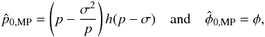 (13)where
h(x) is the Heaviside step function. The Heaviside
function can be motivated by contemplation of Fig. 1a. Equation (13) may be used to
find the maximums in Fig. 1. It is worth noting that this
formula is also expressible as
(13)where
h(x) is the Heaviside step function. The Heaviside
function can be motivated by contemplation of Fig. 1a. Equation (13) may be used to
find the maximums in Fig. 1. It is worth noting that this
formula is also expressible as 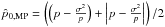 , which may be more practical in
data reduction pipelines, and
, which may be more practical in
data reduction pipelines, and  in terms of the barred
variables.
in terms of the barred
variables.
The goal is to replace these estimators with new ones based on Bayesian ideas and Decision Theory. The ML estimate continues to be relevant in that context because it is equal to some Bayesian estimators when a uniform prior is used.
2.3. The Rice distribution
The Rice distribution (Rice 1945),
R, is the marginal distribution of p over
f,  (14)This integration
may be accomplished using the integral
(14)This integration
may be accomplished using the integral 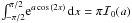 so that
  (15)Here,
ℐ0(x) denotes the zeroth-order modified Bessel function of
the first kind1. It is an even real
function when its argument is real and ℐ0(0) = 1. The Rice
distribution does not depend on or φ
after the integration over φ so they have been dropped from the notation.
(15)Here,
ℐ0(x) denotes the zeroth-order modified Bessel function of
the first kind1. It is an even real
function when its argument is real and ℐ0(0) = 1. The Rice
distribution does not depend on or φ
after the integration over φ so they have been dropped from the notation.
 |
Fig. 2 Two contour plots of the Rice distribution (Eq. (16)). The contours are spaced by 0.1 intervals. The value of
σ is mostly unimportant for
|
In barred variables, the Rice distribution is  (16)This is shown as
a contour plot in Fig. 2a. In this plot,
(16)This is shown as
a contour plot in Fig. 2a. In this plot,
 is plotted
against and
is plotted
against and
 . The
contours are at 0.1 intervals. There are two special points in the plot. A global maximum
of 1/
. The
contours are at 0.1 intervals. There are two special points in the plot. A global maximum
of 1/ is reached at
(1,0) (black dot) and a critical point at
is reached at
(1,0) (black dot) and a critical point at
 (gray
dot) is found if maximums along vertical slices are examined. Recall
(gray
dot) is found if maximums along vertical slices are examined. Recall
 and
and
 . The
maximum along a vertical slice in the interval
. The
maximum along a vertical slice in the interval  lies on the p/σ-axis while for values
greater than
lies on the p/σ-axis while for values
greater than  it lies above the axis. Tracing the maximum of the vertical slices for
 implicitly defines a curve which is given by
  (17)This is the ML
estimator of Simmons & Stewart (1985) (with
a factor of i corrected). ℐ1(x) is the
first-order modified Bessel function of the first kind. It is an odd real function when
its argument is real. Similarly, horizontal slices define a curve via
(17)This is the ML
estimator of Simmons & Stewart (1985) (with
a factor of i corrected). ℐ1(x) is the
first-order modified Bessel function of the first kind. It is an odd real function when
its argument is real. Similarly, horizontal slices define a curve via  (18)This is the
Wardle and Kronberg estimator (Wardle & Kronberg
1974). These are the two dashed curves in the plot. The curve for the horizontal
slice maximums is the one that terminates at the global maximum. The red dotted line is
the Wang estimator from Eq. (13). There is
a significant difference between the Rice distribution-based estimators and the
two-dimensional estimator. For large values of , it
estimates a smaller value of lower than the two
other curves.
(18)This is the
Wardle and Kronberg estimator (Wardle & Kronberg
1974). These are the two dashed curves in the plot. The curve for the horizontal
slice maximums is the one that terminates at the global maximum. The red dotted line is
the Wang estimator from Eq. (13). There is
a significant difference between the Rice distribution-based estimators and the
two-dimensional estimator. For large values of , it
estimates a smaller value of lower than the two
other curves.
Figure 2b plots the Rice distribution with the full range
of when
σ = 1/8. Except near the origin, much of the
probability is distributed in a diagonal linear band that continues uninterrupted until
the maximum value of . Later it will be
seen that the posterior distribution becomes non-linear for large values of polarization.
2.4. The posterior distribution
The distribution given by Eq. (9) is the
distribution of the measured values given true values as input parameters. In practice,
one usually wishes to estimate the true values from the measured values. This is
accomplished through the posterior distribution, B, given by Bayes
Theorem provided one accepts some prior distribution,
 , for
the model parameters. The posterior distribution (for a single measurement) is,
, for
the model parameters. The posterior distribution (for a single measurement) is,
 (19)Care must be taken with
the limits of the p0 integration and it must always be
remembered if one is using the unnormalized, normalized, or barred variables. The barred
version is
(19)Care must be taken with
the limits of the p0 integration and it must always be
remembered if one is using the unnormalized, normalized, or barred variables. The barred
version is 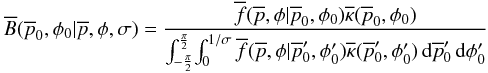 (20)with
 . It is
critical to notice the upper limit of the integration of
is
1/σ, which equals
I0/Σ. It is not infinity as is sometimes
used. In practice, however, many of the integrals over
that occur in
Bayesian polarization equations, tend to be extremely insensitive to the value of
1/σ so long as it is above a value of about 4. Thus,
using infinity as the upper limit often produces a very reasonable approximation. This has
the added advantage that integrals sometimes have explicit closed forms when otherwise
they might not.
. It is
critical to notice the upper limit of the integration of
is
1/σ, which equals
I0/Σ. It is not infinity as is sometimes
used. In practice, however, many of the integrals over
that occur in
Bayesian polarization equations, tend to be extremely insensitive to the value of
1/σ so long as it is above a value of about 4. Thus,
using infinity as the upper limit often produces a very reasonable approximation. This has
the added advantage that integrals sometimes have explicit closed forms when otherwise
they might not.
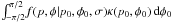
There is great freedom in defining a Bayesian prior. The function is ostensibly required to be a probability distribution. This necessitates that κ(p0,φ0) be non-negative everywhere; however, in most situations, the additional requirement that the distribution be normalizable may be relaxed as the normalization constant cancels. The choice of prior will be further discussed in Sect. 3.
Equation (20) is shown in Figs. 3 and 4 for
I0/Σ = 100 and two different choices of
prior. Figure 3 uses
 and
Fig. 4 uses
and
Fig. 4 uses  . These priors are discussed in
more detail in Sect. 3. Each plot shows several
different values of p/σ. As before,
changing the value of φ merely shifts the distribution along the
φ0 axis so φ = 0 has been used. In
Figs. 2.5 and 4a, p/σ = 0 and there is no
preference for any over another. In
Figs. 2.5 and 4b,
p/σ = 0.5. Here a probability
bubble is beginning to form. In Figs. 2.5 and 4c,
p/σ = 2.0 and the probability bubble
is now fairly mature. The panels of Fig. 4 are similar.
Notice that Fig. 3 is nearly identical to the distribution
plotted in Fig. 1. There is a very weak dependence of
. These priors are discussed in
more detail in Sect. 3. Each plot shows several
different values of p/σ. As before,
changing the value of φ merely shifts the distribution along the
φ0 axis so φ = 0 has been used. In
Figs. 2.5 and 4a, p/σ = 0 and there is no
preference for any over another. In
Figs. 2.5 and 4b,
p/σ = 0.5. Here a probability
bubble is beginning to form. In Figs. 2.5 and 4c,
p/σ = 2.0 and the probability bubble
is now fairly mature. The panels of Fig. 4 are similar.
Notice that Fig. 3 is nearly identical to the distribution
plotted in Fig. 1. There is a very weak dependence of
 on
σ that becomes larger for larger values of
p0. If p0 were plotted near the
maximum, the plots would differ radically. When
1/σ → ∞, the plots do become identical. The similarity
(and differences) will be discussed later in conjunction with the one-dimensional,
marginalized version of this plot.
on
σ that becomes larger for larger values of
p0. If p0 were plotted near the
maximum, the plots would differ radically. When
1/σ → ∞, the plots do become identical. The similarity
(and differences) will be discussed later in conjunction with the one-dimensional,
marginalized version of this plot.
2.5. Simple Bayesian estimators
Bayesian estimators based on the mean, median, and mode can be defined for the posterior distribution.
The mode estimator (usually called the MAP or maximum a posteriori estimate) is the maximum of the posterior distribution. If any delta function is used in the prior, this causes delta functions to appear in the posterior distribution, which trumps any finite maximum of the posterior distribution and renders the mode estimate somewhat useless without further modification. If no delta functions and a uniform prior is used, then the mode estimate is the same as the ML estimate (Eq. (12)).
The median estimator,  ,
is the value such that
,
is the value such that 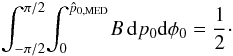 (21)This estimator will
usually have to be found numerically. A median estimator
(21)This estimator will
usually have to be found numerically. A median estimator
 is usually easy to find from symmetry considerations but for our parameter space must be
defined as
is usually easy to find from symmetry considerations but for our parameter space must be
defined as 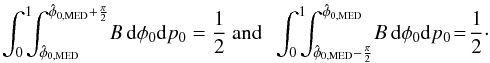 (22)Under special
circumstances,
may not be unique but after a non-zero measurement of p, it will
generally be the case that it is.
(22)Under special
circumstances,
may not be unique but after a non-zero measurement of p, it will
generally be the case that it is.
The mean estimators are the values  (23)and
 (24)These three
estimators will be different in general.
(24)These three
estimators will be different in general.
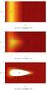 |
Fig. 3 Contour plots of |

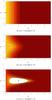 |
Fig. 4 Contour plots of |

2.6. Bayesian decision theory
The posterior distribution contains all information about the relative likelihood of the model parameters. It represents what has been learned from the observation. For many problems it is usually desired to summarize the posterior distribution by a few statistics such as an estimate of the “best” value and some confidence interval (often called “credible sets” in this context). In Bayesian Decision and Estimation Theory determining the “best” estimate of the model parameters requires defining a loss function and a decision rule (there are many good standard texts offering much more detail such as Berger 1985; and Robert 1994). The loss function, L, assigns a weight to deviations from the true value such that measured values that are far away from it incur a greater penalty than those that are closer. The decision rule assigns an estimate of the true value based upon the data, which will usually be the estimate that minimizes the expected posterior probable loss.
Deciding upon a loss function is one of the toughest parts of a Bayesian analysis. The three most common are squared-error loss, absolute deviation loss, and the “0–1” loss. These loss functions have as their solutions for each variable the mean, median, and mode values of the posterior, respectively (Robert 1994).
The squared-deviation loss function for the polarization problem may be defined as the
squared distance between the true value
(q0,u0) and the
best estimate
(qa,ua)
under a Euclidean metric (scaled by σ2),  (25)Transforming Eq. (25) to polar coordinates gives,
 (26)The posterior
expected loss, Z, under B is
(26)The posterior
expected loss, Z, under B is
 (27)Loss can be
minimized by solving
(27)Loss can be
minimized by solving  and
and
 and checking that the solution
is a minimum via the second derivative test. These two equations are difficult to solve
completely but it can be shown that if
κ(p0,φ0) = κ(p0)
then
and checking that the solution
is a minimum via the second derivative test. These two equations are difficult to solve
completely but it can be shown that if
κ(p0,φ0) = κ(p0)
then 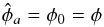 (28)and
 (29)are a
solution and
(29)are a
solution and  when
pa,p0 > 0
so the solutions are a minimum.
when
pa,p0 > 0
so the solutions are a minimum.
The absolute loss function is  (30)It will be assumed that
the usual median estimators in polar coordinates are in fact a solution to this loss
function.
(30)It will be assumed that
the usual median estimators in polar coordinates are in fact a solution to this loss
function.
The “0–1” loss function is 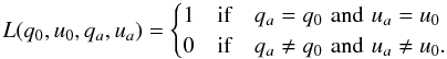 (31)It
will also be assumed that the mode is the solution of this loss function. When the prior
contains a delta function, this estimator is not very useful.
(31)It
will also be assumed that the mode is the solution of this loss function. When the prior
contains a delta function, this estimator is not very useful.
2.7. Posterior odds
An analog of hypothesis testing in Bayesian analysis is the comparison of posterior odds.
In the simplest case, suppose one wishes to test the hypothesis that the model parameters
lie in some subset Θ1 of the parameter space. This is accomplished by
integrating the posterior distribution over the subset. If the probability is greater than
50%, the hypothesis is accepted. If it is less than 50%, it is rejected. The simplicity of
these tests is one of the benefits of the Bayesian approach. The subset need not consist
of more than a single point but in that case the associated probability will usually be
infinitesimal unless distributions are allowed for priors. In the next section, priors
will be introduced that use a delta function at the origin to represent the probability
that a source has negligible polarization. After the measurement, one may compute the
posterior odds for the origin (a single point) to test if the measurement is consistent
with zero. One of the benefits of
is that it naturally performs this test for a delta function at the origin.
Two probabilities are of interest, the probability that p0 is
zero and the probability that p0 is greater than zero. In
mathematical form, 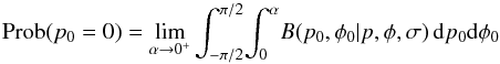 (32)and
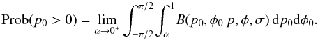 (33)Since the
distribution is normalized, only Eq. (32)
need actually be calculated because
Prob(p0 = 0) + Prob(p0 > 0) = 1.
If
Prob(p0 = 0) > 1/2,
then it is more likely the source has negligible than appreciable polarization. If
Prob(p0 = 0) < 1/2,
then it is more likely the source has appreciable than negligible polarization.
(33)Since the
distribution is normalized, only Eq. (32)
need actually be calculated because
Prob(p0 = 0) + Prob(p0 > 0) = 1.
If
Prob(p0 = 0) > 1/2,
then it is more likely the source has negligible than appreciable polarization. If
Prob(p0 = 0) < 1/2,
then it is more likely the source has appreciable than negligible polarization.
It is now time to discuss choosing a prior so that these equations may be used.
3. Elicitation of priors
In Bayesian statistics, the choice of the prior distribution is non-trivial and can be very controversial because it is frequently subjective and based on previous experience for the problem at hand. The purpose of the prior density is to represent knowledge of the model parameters before an experiment. One common situation is where one has no prior knowledge of their values and wishes to construct a prior to represent this ignorance. Such priors are called “objective”. Constructing objective priors can be extremely subtle. The Bertrand Paradox illustrates that the method of producing or defining a “random” value can have important consequences for the resulting probability distributions (Bertrand 1888). In general, the solution to the Bertrand Paradox is that “real randomness” requires certain translation and scaling invariance properties (Jaynes 1973; Tissier 1984; Di Porto et al. 2010). In practice, such objective priors may contain too little information to satisfactorily model the phenomena being studied.
In general, the polarization state of an unresolved source at a particular wavelength is described by a point of the Poincaré sphere, which is the three-dimensional set of the physically possible values for the q, u, and v Stokes parameters given an intensity. An assumption was made in the introduction that circular polarization is negligible. This is a physical assumption which influences the meaning of the polarization state of a “random” source. The resulting q − u distribution of random sources is not to be confused with the expected q − u distribution of a random source whose v component was ignored. For a uniform distribution of points within the Poincaré sphere, this latter distribution would be the density distribution obtained by projection onto the q − u plane, which would have a larger density near the origin. This distribution is important and interesting but its three-dimensional motivation is somewhat outside two-dimensional scope of this work. A brief discussion of it is given in Appendix B.
Investigation is still required into the meaning of “randomness” even under just the V = 0 point-of-view. It is necessary to understand what role the choice of coordinates plays and how “uniform” does not imply “random”.
3.1. Uniform prior in Cartesian coordinates (the Jeffreys prior)
The prior most likely to coincide with a person’s intuitive notion of a “random point” in
the unit disk is a uniform distribution in
q0-u0 coordinates is
 (34)In polar
coordinates, this is equivalent to
(34)In polar
coordinates, this is equivalent to 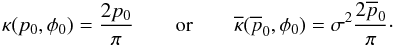 (35)The barred versions are
always
(35)The barred versions are
always 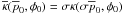 . Both distributions are
normalized. Random points generated using this distribution have an expected density that
is constant across the unit disk (see Fig. 5a). One
aspect of this prior is that a randomly generated point will generally be more likely to
have a strong polarization than a weak one because an annulus associated with a large
radius has more area than for a smaller radius.
. Both distributions are
normalized. Random points generated using this distribution have an expected density that
is constant across the unit disk (see Fig. 5a). One
aspect of this prior is that a randomly generated point will generally be more likely to
have a strong polarization than a weak one because an annulus associated with a large
radius has more area than for a smaller radius.
It can be shown that the prior given by Eq. (34) is the normalized Jeffreys prior for the polarization problem. The Jeffreys prior is an objective prior constructed from the square root of the determinate of the Fisher information matrix (Jeffreys 1939, 1946; Robert et al. 2009a,b). One of the features of the Jeffreys prior is that it is invariant under a re-parametrization. As an objective prior, the Jeffreys prior is in some sense the prior desired when absolutely no previous knowledge of the model parameters is known.
While the objectivity of this prior is admirable, in practice, most astronomical sources are not expected to have very large polarizations (masers can be a notable exception); so, in many cases, it is undesirable that the polarization be more likely to be large than small. In this respect, this prior may not be a good choice for some astrophysical observations despite its objectivity: it simply contains too little information to be suitable and overestimates our lack of knowledge and previous experience.
 |
Fig. 5 A comparison of “random” points generated with the Jeffreys prior and the uniform polar prior. |
3.2. Uniform prior in polar coordinates
The uniform prior in polar coordinates captures some features that are usually desired
for astronomical sources than the previous case. Its (normalized) formula is 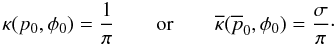 (36)While this prior
may be “uniform” in p0 − φ0 space
(see Fig. 5b), it is definitely not uniform in
q0 − u0 space. In fact, in that
space, the density of points produced randomly by this prior increases near the origin, as
is shown in Fig. 5c. This is a subjective prior in the
sense that it prefers points closer to the origin.
(36)While this prior
may be “uniform” in p0 − φ0 space
(see Fig. 5b), it is definitely not uniform in
q0 − u0 space. In fact, in that
space, the density of points produced randomly by this prior increases near the origin, as
is shown in Fig. 5c. This is a subjective prior in the
sense that it prefers points closer to the origin.
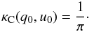
3.3. The addition of a delta term at the origin
One subtle feature of the previous priors is that they do not allow for a finite probability that an object’s polarization is exactly zero. Instead there is only a finite chance that the polarization will be in some interval that includes zero. A Dirac delta function at the origin may be used to allow for the possibility that an object truly has zero polarization. “Exactly zero” polarization may be interpreted as equivalent to the statement that there is a large probability that the polarization is negligible. In this case, the delta function then becomes just a mathematical tool to replace a probability density that rises extremely sharply at the origin in such a way to bound an appreciable probability.
When one is investigating if some class of objects are polarized, it
seems reasonable to assign a 50% chance to the probability that the object is unpolarized
and a 50% chance to it being polarized. More generally, the percentage can be
parametrized, such that the probability of zero polarization is A and
greater than zero polarization is (1 − A). Let the prior consists of two
components: a normalized delta function term at the origin,
 , and a
normalized non-delta function term,
, and a
normalized non-delta function term,  . The
general form for the prior can now be written as
. The
general form for the prior can now be written as  (37)or
  (38)The delta term must be
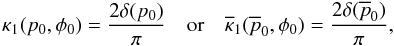 (39)respectively. The
two versions in Eq. (39) have the same
form because the delta function transforms in a way that cancels the σ’s
that typically will appear in the barred version. Notice too that the
p0-delta function occurs at the lower limit of the
p0 integration. This is a somewhat quirky situation but by
remembering that delta functions are constructed as a limit of a sequences of functions it
is easily seen that
(39)respectively. The
two versions in Eq. (39) have the same
form because the delta function transforms in a way that cancels the σ’s
that typically will appear in the barred version. Notice too that the
p0-delta function occurs at the lower limit of the
p0 integration. This is a somewhat quirky situation but by
remembering that delta functions are constructed as a limit of a sequences of functions it
is easily seen that 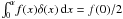 for
α > 0. Taking into account the factors of
one-half that arise in this way, it can be shown that Eqs. (38) and (39) are both
normalized properly2. A delta function could also be
placed at any other point in the disk of physically possible values but the origin is
unique as it is the only case that preserves rotational symmetry.
for
α > 0. Taking into account the factors of
one-half that arise in this way, it can be shown that Eqs. (38) and (39) are both
normalized properly2. A delta function could also be
placed at any other point in the disk of physically possible values but the origin is
unique as it is the only case that preserves rotational symmetry.
The previous priors with the addition of a delta term become
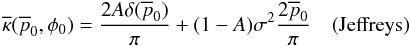 (40)and
 (41)These priors simplify
to the more typical cases when A = 0. The delta term however is an
interesting addition. It is only with the addition of the delta term and the use of the
median estimator that one is allowed to state the source is consistent with no
polarization from the posterior distribution. It seems most reasonable to assign
A the value 0.5 when it is unknown if the source is polarized. Another
interesting choice is
(41)These priors simplify
to the more typical cases when A = 0. The delta term however is an
interesting addition. It is only with the addition of the delta term and the use of the
median estimator that one is allowed to state the source is consistent with no
polarization from the posterior distribution. It seems most reasonable to assign
A the value 0.5 when it is unknown if the source is polarized. Another
interesting choice is  .
This value causes the Prob(p0 = 0) for the prior to be equal
to the probability density of the non-delta function component. There is a temptation to
say that it recaptures some translation invariance properties that are otherwise lost upon
the introduction of the delta term. It is unclear to the author if this has any
mathematical significance or indeed how to justify a particular choice of
A in general. Using A = 0 is the most conservative
choice and is probably the most appropriate in many experiments unless a non-zero
A is explicitly required. A non-zero value of A, as
will be seen, can cause the median estimator of to be zero below
some critical value of . One way of
interpreting this is that the median estimator determines what value of polarization must
be measured to convince a person who is skeptical of polarization with degree
A that a source is actually polarized. Ultimately, it is up to the
researcher to decide the best prior for the experiment.
.
This value causes the Prob(p0 = 0) for the prior to be equal
to the probability density of the non-delta function component. There is a temptation to
say that it recaptures some translation invariance properties that are otherwise lost upon
the introduction of the delta term. It is unclear to the author if this has any
mathematical significance or indeed how to justify a particular choice of
A in general. Using A = 0 is the most conservative
choice and is probably the most appropriate in many experiments unless a non-zero
A is explicitly required. A non-zero value of A, as
will be seen, can cause the median estimator of to be zero below
some critical value of . One way of
interpreting this is that the median estimator determines what value of polarization must
be measured to convince a person who is skeptical of polarization with degree
A that a source is actually polarized. Ultimately, it is up to the
researcher to decide the best prior for the experiment.
Under Eq. (38), the posterior
distribution reduces to  (42)Figures 3 and 4 were special cases of this
formula.
(42)Figures 3 and 4 were special cases of this
formula.
3.4. Other constructions
Bayesian statisticians have invented a number of other techniques for constructing priors such as using conjugate families and building hierarchical models. These are not covered.
4. Marginal distributions of polarization magnitude
The marginal posterior distribution, S, of p0
over B is given by  (43)The denominator of
B is a function of p and φ only and may
be pulled through the integral. The numerator becomes
(43)The denominator of
B is a function of p and φ only and may
be pulled through the integral. The numerator becomes
 . No further
simplifications can be made unless a prior is chosen. While not necessary, it will
frequently be the case that priors for a first measurement are independent of angle, that
is,
κ(p0,φ0) = κ(p0).
If so, then it is easy to show that
. No further
simplifications can be made unless a prior is chosen. While not necessary, it will
frequently be the case that priors for a first measurement are independent of angle, that
is,
κ(p0,φ0) = κ(p0).
If so, then it is easy to show that 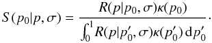 (44)(An integration of the
sampling function under consideration,
(44)(An integration of the
sampling function under consideration,  , arrives
at the same result, Eq. (15), regardless if
the integration is over φ0 or φ due to the
symmetry in those variables). The resulting new posterior, which may be treated as a prior
for the next measurement, will not, in general, be independent of angle. The condition
, arrives
at the same result, Eq. (15), regardless if
the integration is over φ0 or φ due to the
symmetry in those variables). The resulting new posterior, which may be treated as a prior
for the next measurement, will not, in general, be independent of angle. The condition
 therefore
does not extend to multiple measurements. Those are not the focus of this investigation and
none of the κ-priors examined so far vary with angle. Equation (44) turns out to be exactly the same form as the
posterior Rice distribution, which is now examined.
therefore
does not extend to multiple measurements. Those are not the focus of this investigation and
none of the κ-priors examined so far vary with angle. Equation (44) turns out to be exactly the same form as the
posterior Rice distribution, which is now examined.
4.1. Posterior Rice distributions
Vaillancourt (2006) uses a Bayesian approach to argue for the use of the posterior Rice distribution to calculate the maximum likelihood and error bars on measured polarization. This special case was the motivation for the more general theory of this paper.
Introduce new one-dimensional prior τ(p0).
The posterior Rice distribution, ρ, is 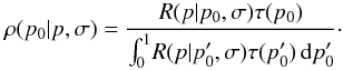 (45)The conversion to barred
priors is given by
(45)The conversion to barred
priors is given by  . The barred version of the
formula is
. The barred version of the
formula is 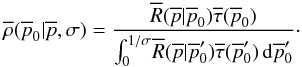 (46)The objective prior in
one dimension is τ(p0) = 1 so technically the
one-dimensional Jeffreys prior and the uniform polar prior are the same. As can be seen
from Eqs. (44) and (45), when
κ(p0) is independent of angle,
S and ρ have the same form with
κ(p0) playing the role of
τ(p0). The “one-dimensional” version of the
two-dimensional Jeffreys prior is
τ(p0) = 2p0 and
the one-dimensional version of the two-dimensional uniform polar prior is
τ(p0) = 1. There is only an immaterial
factor of 1/π difference between
κ(p0) and
τ(p0). In a slight abuse of terminology,
τ(p0) = 2p0
will still be called the “Jeffreys prior” despite switching to the one-dimensional
notation. The two-dimensional theory is still within context because of Eq. (44). In barred variables, the priors are
(46)The objective prior in
one dimension is τ(p0) = 1 so technically the
one-dimensional Jeffreys prior and the uniform polar prior are the same. As can be seen
from Eqs. (44) and (45), when
κ(p0) is independent of angle,
S and ρ have the same form with
κ(p0) playing the role of
τ(p0). The “one-dimensional” version of the
two-dimensional Jeffreys prior is
τ(p0) = 2p0 and
the one-dimensional version of the two-dimensional uniform polar prior is
τ(p0) = 1. There is only an immaterial
factor of 1/π difference between
κ(p0) and
τ(p0). In a slight abuse of terminology,
τ(p0) = 2p0
will still be called the “Jeffreys prior” despite switching to the one-dimensional
notation. The two-dimensional theory is still within context because of Eq. (44). In barred variables, the priors are
 and
and
 , respectively.
4.1.1. Mean estimator for the posterior Rice distribution
The mean estimator,  ,
is given by
,
is given by 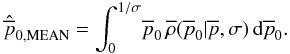 (47)Its value is always
greater than zero for any given and will
usually have to be found numerically.
(47)Its value is always
greater than zero for any given and will
usually have to be found numerically.
4.1.2. Median estimator for the posterior Rice distribution
The median estimator,  ,
for the posterior Rice distribution is the value of the upper integrand such that
,
for the posterior Rice distribution is the value of the upper integrand such that
 (48)This expression
will also have to be solved numerically in most cases.
(48)This expression
will also have to be solved numerically in most cases.
4.2. Selected plots of the posterior Rice distribution
Figure 6 shows two versions of the posterior Rice
distribution using the Jeffreys prior, . Figure 6a shows the distribution near the origin and assuming
1/σ = 100. Figure 6b
shows the full range of assuming
1/σ = 8. This figure exhibits several key results.
For the Jeffreys prior, the posterior Rice distribution is similar to just the transpose
of the Rice distribution. This similarity breaks down at values of
near or
exceeding the maximum value of . The mean (black)
and median (blue) estimator curves, are very similar. They are also similar to the
(transposed) one-dimensional Rice distribution estimator curves but that similarity also
breaks down at near the maximum value of .
 |
Fig. 6 Two contour plots of the posterior Rice distribution (Eq. (46)) with
|

 |
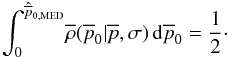
Fig. 7 Two contour plots of the posterior Rice distribution (Eq. (46)) with
|

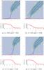 |
Fig. 8 These four panels show the posterior distribution
|

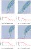 |
Fig. 9 These four panels show the posterior distribution
|

Figure 7 uses and two different values of
σ. Figure 7a is nearly the same
plot as presented in Vaillancourt (2006), which
used τ(p0) = 1 and the unstated assumption
that I0/Σ → ∞, which allows direct
integration of the denominator of Eq. (46)
at the expense of having an unnormalizable prior. While this approximation will be
acceptable most of the time when the signal-to-noise is large, it is unphysical. The true
value of cannot exceed
1/σ
(=I0/Σ), which is finite. This is best
seen by plotting the full range of as is done in
Fig. 7b for
I0/Σ = 8 (a small value). There it is
seen that for values of that are
near or greater than the maximum possible value of (8 in this case),
the probability density function “crowds up” near the maximum value. This time the mean
(black) and median (blue) curves are rather different. The median curve prefers value
closer to  . The
median estimator seems to be a better statistic in this case as the mean estimator curve
is affected too much by outlier possibility.
. The
median estimator seems to be a better statistic in this case as the mean estimator curve
is affected too much by outlier possibility.
A delta term may also be added to the prior as was previously motivated. Let
τ(p0) = Aτ1(p0) + (1 − A)τ2(p0),
where τ1(p0) is normalized a delta
term at the origin and τ2(p0) is a
normalized component without any delta terms. The normalized barred prior is
 . This time
τ1(p0) = 2δ(p0)
and
. This time
τ1(p0) = 2δ(p0)
and  . Under this prior, Eq. (46) reduces to
 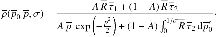 (49)Here, the function
arguments have been dropped for space. For the two-component prior, the definition of the
median estimator (Eq. (48)) leads to the
following expression
(49)Here, the function
arguments have been dropped for space. For the two-component prior, the definition of the
median estimator (Eq. (48)) leads to the
following expression 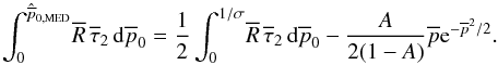 (50)Figures 8 and 9 show Eq. (49) for the Jeffreys and uniform priors,
respectively, and four different combination of values of A and
σ each. The red, dashed lines at
are a
reminder that Eq. (49) contains a delta
term that cannot be plotted in the usual fashion. Finite probability is attached to each
point along the red line and is graphed beneath each contour plot. This is critical to
fully understand these plots. Several new features are seen for non-zero
A. In Fig. 8 for the Jeffreys prior,
the probability band seems to bend towards the -axis
(Fig. 8a) but in actuality abruptly turns and heads
towards the -axis (Fig. 8b). This behavior is however strongly damped by residual
probability that the polarization is actually zero (as in Figs. 8c and d). Figure 9 for the uniform polar prior
is similar except this time the probability band, after heading towards the
-axis as
well, turns towards the origin if the behavior is not damped by the probability that the
polarization is zero (as in Figs. 9c and d).
(50)Figures 8 and 9 show Eq. (49) for the Jeffreys and uniform priors,
respectively, and four different combination of values of A and
σ each. The red, dashed lines at
are a
reminder that Eq. (49) contains a delta
term that cannot be plotted in the usual fashion. Finite probability is attached to each
point along the red line and is graphed beneath each contour plot. This is critical to
fully understand these plots. Several new features are seen for non-zero
A. In Fig. 8 for the Jeffreys prior,
the probability band seems to bend towards the -axis
(Fig. 8a) but in actuality abruptly turns and heads
towards the -axis (Fig. 8b). This behavior is however strongly damped by residual
probability that the polarization is actually zero (as in Figs. 8c and d). Figure 9 for the uniform polar prior
is similar except this time the probability band, after heading towards the
-axis as
well, turns towards the origin if the behavior is not damped by the probability that the
polarization is zero (as in Figs. 9c and d).
The mean and median estimator curves in Figs. 8 and 9 have changed with the introduction of a non-zero
A. The mean curve is “pulled” more towards the
-axis at
small values of for larger
values of A or smaller values of σ. The median curve has
a totally new feature: it intercepts the -axis at a
critical value,  , and is zero
for smaller values. This occurs when the right-hand side of Eq. (50) equals zero. Tables of some critical
values, including those corresponding to the figures, are presented in Appendix A.
, and is zero
for smaller values. This occurs when the right-hand side of Eq. (50) equals zero. Tables of some critical
values, including those corresponding to the figures, are presented in Appendix A.
When A = 0 and σ = 0.01, a contour plot of Eq. (49) for the Jeffrey prior reproduces
Fig. 6a. This plot resembles the Rice distribution
in Fig. 2a, only transposed! Figure 8b is a good example of the transitional form that occurs in the contour
shape between the standard A = 0 form and the form seen for larger values
of A and/or smaller values of σ. This is an important
result. It means that the Rice distribution results can effectively be transposed to find
best estimates of for small values
of polarization when 1/σ → ∞.
When A = 0 and σ = 0.01, a contour plot of Eq. (49) for the uniform prior reproduces Fig. 7a. There is no delta function and the global maximum of this distribution occurs at the origin. The wrench-like shape characteristic of this plot arises from small values of A for a given value of σ. Figure 9b is a good example of the transitional form.
All the usual mathematical machinery may now be applied to
 to produce estimators for
given a measured
value of .
to produce estimators for
given a measured
value of .
Previously “bias corrections” were performed on measurements at low signal-to-noise to make them closer to zero. As is seen in the figures with A = 0, the mean and median estimators seem to act for very small values of p like a “bias correction” that goes the wrong way! (The median estimator curves with p-axis intercepts are an exception.) Bias corrections should not be used. A non-zero value for the estimate of p0 even when p = 0 is not a deficiency with the estimators. It is a result that can be understood intuitively when all possible values of p0 and φ0 that could have produced a given p and φ are considered.
5. Marginal distributions of polarization angle
The marginal posterior distribution, T, of φ0
is given by  (51)As before, the
denominator of B is a function of p and φ
only and may be pulled through the integral. The numerator becomes
(51)As before, the
denominator of B is a function of p and φ
only and may be pulled through the integral. The numerator becomes
 . If the prior is a
function of p0 to some non-negative integer power
n (i.e.,
. If the prior is a
function of p0 to some non-negative integer power
n (i.e.,  , there appears to
exist a family of solutions via repeated integration by parts. Explicit solutions were found
up to n = 10 using the computer algebra system Mathematica. Beyond
n = 1, these solutions quickly become impractically large.
, there appears to
exist a family of solutions via repeated integration by parts. Explicit solutions were found
up to n = 10 using the computer algebra system Mathematica. Beyond
n = 1, these solutions quickly become impractically large.
The marginal distribution, G, of φ over
f has been investigated by several authors (Vinokur 1965; Clarke & Stewart
1986; Naghizadeh-Khouei & Clarke
1993). Its defining formula in terms of the sky angle is
 Unfortunately, the
solution to this equation in Clarke & Stewart
(1986) has some sign mistakes and the derivation in Appendix B of Naghizadeh-Khouei & Clarke (1993) confuses the
sky angle, φ, with the angle in the q − u
plane, θ. It is worth explicitly stating both versions to avoid confusion:
Unfortunately, the
solution to this equation in Clarke & Stewart
(1986) has some sign mistakes and the derivation in Appendix B of Naghizadeh-Khouei & Clarke (1993) confuses the
sky angle, φ, with the angle in the q − u
plane, θ. It is worth explicitly stating both versions to avoid confusion:
![Mathematical equation: \begin{equation} G(\phi{}|p_0,\phi{}_0,\sigma{}) = \frac{1}{\sqrt{\pi{}}} \left(\frac{1}{\sqrt{\pi{}}} + \eta{}_0 {\rm e}^{\eta{}^2_0} \left[1+\operatorname{erf}(\eta{}_0)\right] \right) {\rm e}^{-\frac{p^2_0}{2\sigma{}^2}} \label{eq:G} \end{equation}](/articles/aa/full_html/2012/02/aa15785-10/aa15785-10-eq289.png) (52)and
(52)and
![Mathematical equation: \begin{equation} G'(\theta{}|p_0,\theta{}_0,\sigma{}) = \frac{1}{2\sqrt{\pi{}}} \left(\frac{1}{\sqrt{\pi{}}} + \eta{}'_0 {\rm e}^{\eta{}'^2_0} \left[1+\operatorname{erf}(\eta{}'_0)\right] \right) {\rm e}^{-\frac{p^2_0}{2\sigma{}^2}}, \end{equation}](/articles/aa/full_html/2012/02/aa15785-10/aa15785-10-eq290.png) (53)where
(53)where
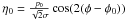 and
and
 . It is useful to notice that the
distribution is symmetric about φ0 and using a value of
φ0 different than zero only translates the distribution along
the angular axis. Therefore when calculating confidence intervals, only
φ0 = 0 need be used. Unlike the Rice distribution, which is
independent of the angular variable, this distribution depends on
p0. G is normalized (i.e.,
. It is useful to notice that the
distribution is symmetric about φ0 and using a value of
φ0 different than zero only translates the distribution along
the angular axis. Therefore when calculating confidence intervals, only
φ0 = 0 need be used. Unlike the Rice distribution, which is
independent of the angular variable, this distribution depends on
p0. G is normalized (i.e.,
 ).
).
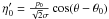
The distribution T cannot in general be related to G as S was to R through ρ, even if the prior is independent of angle, because f lacks the symmetry in p and p0 that it has for φ and φ0. T and G may have different form. If however κ(p0,φ0) ∝ p0, as with the Jeffreys prior, it is easy to show that T → G as 1/σ → ∞.
Figure 10 compares T to
G for the Jeffreys prior, i.e.,  , and
I0/Σ = 100 and three different
signal-to-noise values. As expected, the T distribution and the
G distribution are almost identical because
1/σ is fairly large. The two sets of curves overlap in
the figure but the T curves are not precisely identical to the
G curves. The difference between the T and
G curves is larger if 1/σ is small or
for polarization measurements near 1/σ. In practice, the
classical error bars for the angle based on G are perfectly acceptable
under this prior.
, and
I0/Σ = 100 and three different
signal-to-noise values. As expected, the T distribution and the
G distribution are almost identical because
1/σ is fairly large. The two sets of curves overlap in
the figure but the T curves are not precisely identical to the
G curves. The difference between the T and
G curves is larger if 1/σ is small or
for polarization measurements near 1/σ. In practice, the
classical error bars for the angle based on G are perfectly acceptable
under this prior.
Figure 11 compares T to
G for the case of a uniform polar prior, i.e.,
 , and
I0/Σ = 100. In the figure,
T (blue) is plotted for φ = 0 and
p/σ = 0.5 (dotted), 1.0 (solid), 2.0
(dashed) and G (red) is plotted for and
p0/σ = 0.5 (dotted), 1.0
(solid), 2.0 (dashed). The figure clearly demonstrates that using G, the
non-Bayesian formula, to compute errors bars results in errors bars that are too small. This
is especially important when the polarization degree to σ ratio is about
one.
, and
I0/Σ = 100. In the figure,
T (blue) is plotted for φ = 0 and
p/σ = 0.5 (dotted), 1.0 (solid), 2.0
(dashed) and G (red) is plotted for and
p0/σ = 0.5 (dotted), 1.0
(solid), 2.0 (dashed). The figure clearly demonstrates that using G, the
non-Bayesian formula, to compute errors bars results in errors bars that are too small. This
is especially important when the polarization degree to σ ratio is about
one.
If a delta term is added to the priors as was done with the polarization magnitude plots,
the result can roughly be described by saying that the distribution is scaled by
(1 − A) and it is then shifted upwards by a constant of
A/π. This constant shift occurs
because the origin has an indeterminate angle. The equation in barred variables is
 (54)When
A = 1.0, the distribution is flat with value
1/π, as it must be to be normalized.
(54)When
A = 1.0, the distribution is flat with value
1/π, as it must be to be normalized.
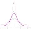 |
Fig. 10 This plot compares the classical angle distribution,
G(φ|p0,φ0,σ),
to the Bayesian distribution,
T(φ0|p,φ,σ), with
|

 |
Fig. 11 This plot compares the classical angle distribution,
G(φ|p0,φ0,σ)
(red), to the Bayesian distribution,
T(φ0|p,φ,σ) (blue),
with |

6. Summary of derivations
Figure 12 is a flow chart to help remember the relationships among the many distributions presented. All the main functions result from a change of variables, Bayes Theorem, or marginalization (denoted by “Marg.” in the figure). Attempts were made to remain consistent with the function names used in previous published papers when possible.
7. Confidence intervals (aka credible sets)
All the pieces needed to construct confidence intervals (known as “credible sets” in
Bayesian statistics) for p0 and
have been given. In
general, these sets will be two-dimensional. Usually they will be constructed so as to
contain the “best” estimate ( and
and  )
that was found. In practice, especially with polarimetric spectra, using two-dimensional
sets as “error bars” is impossible. In these cases, the marginal distributions,
T and S, may be used to construct error bars.
)
that was found. In practice, especially with polarimetric spectra, using two-dimensional
sets as “error bars” is impossible. In these cases, the marginal distributions,
T and S, may be used to construct error bars.
High-quality confidence interval tables, suitable for use in data reduction pipelines, will be the subject of a future paper.
8. Conclusion
A foundation for a Bayesian treatment of polarization measurements has been presented based when V = 0. The treatment covers the regime where the measured polarization has large or small Stokes parameters but all the intensities that were used in the calculation of the Stokes parameters are large enough that Poisson statistics is unimportant. This justifies the use of a gaussian approach for the Stokes parameters’ error.
A Bayesian analysis of polarization allows the observer some freedom in choosing a prior and loss function. These should be stated and justified when presenting one’s results. In particular, the importance of choosing an appropriate prior has been stressed.
The transposed Rice distribution is intimately connected with the posterior distribution with a two-dimensional Jeffreys prior. As 1/σ → ∞, the distributions are the same. The classical angular distribution is also the same as the posterior angular distribution in this limit. A uniform polar prior may be better for sources with small expected polarization. In this case, the posterior distributions are rather different than the classical ones.
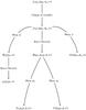 |
Fig. 12 This figure is a flow chart to help remember the relationships between the distributions presented. “Marg.” stands for marginalization over the accompanying variable. |
Further advances may be made by generalizing the analysis to include ellipsoidal, perhaps even correlated, distributions for Q and U, Poisson statistics, circular polarization, or repeated measurements. Monte Carlo methods will likely be necessary to handle the integrations for more general approaches. Polarimetric spectra and time series data that involve measurements that are not independent and may be highly correlated; modeling the wavelength-dependence or time-evolution could further improve results in those situations.
The results presented have focused on the interpretation of the quantities
p0 and φ0 as polarization degree
and angle but the formulas are applicable to any application that uses a bounded radial
function of the form  ,
where x and y are measured with equal gaussian error.
,
where x and y are measured with equal gaussian error.
Some papers in the literature use Bessel functions,
 ,
instead of modified Bessel functions, ℐ. This introduces distracting
complex factors of i into the equations. It is worth noting that
,
instead of modified Bessel functions, ℐ. This introduces distracting
complex factors of i into the equations. It is worth noting that
 and
and  to aid in reading those papers.
This idea of delta functions on boundaries (or even boundaries of boundaries) helps motivate and generally requires the concept of Lebesgue density. Extensions of this paper to include circular polarization, V, would have to be careful to get the Lebesgue density factors correct.
Acknowledgments
The authors acknowledge support from the Millennium Center for Supernova Science (MCSS) through grant P10-064-F funded by “Iniciativa Científica Milenio”. The contour plots were generated using computer algebra system Mathematica (version 7.01.0). The authors wish to thank Alejandro Clocchiatti and Lifan Wang for helpful discussion and the anonymous referee for valuable comments.
References
- Berger, J. O. 1985, Statistical Decision Theory and Bayesian Analsyis, 2nd ed. (Springer) [Google Scholar]
- Bertrand, J. 1888, Calcul des probabilités (Paris: Gauthier-Villars) [Google Scholar]
- Clarke, D., & Stewart, B. G. 1986, Vist. Astron., 29, 27 [NASA ADS] [CrossRef] [Google Scholar]
- Clarke, D., Stewart, B. G., Schwarz, H. E., & Brooks, A. 1983, A&A, 126, 260 [NASA ADS] [Google Scholar]
- del Toro Iniesta, J. C. 2003, Introduction to Spectropolarimetry (Cambridge University Press) [Google Scholar]
- Di Porto, P., Crosignani, B., Ciattoni, A., & Liu, H. C. 2010 [arXiv:1008.1878] [Google Scholar]
- Jaynes, E. T. 1973, Foundations of Physics, 3, 477 [NASA ADS] [CrossRef] [Google Scholar]
- Jeffreys, H. 1939, Theory of probability (Oxford University Press) [Google Scholar]
- Jeffreys, H. 1946, Proc. Royal Society of London Series A, Mathematical and Physical Sciences, 186, 453 [Google Scholar]
- Keller, C. U. 2002, in Astrophysical Spectropolarimetry, ed. J. Trujillo-Bueno, F. Moreno-Insertis, & F. Sánchez, 303 [Google Scholar]
- Landi Degl’Innocenti, E. 2002, in Astrophysical Spectropolarimetry, ed. J. Trujillo-Bueno, F. Moreno-Insertis, & F. Sánchez, 1 [Google Scholar]
- Maronna, R., Feinstein, C., & Clocchiatti, A. 1992, A&A, 260, 525 [NASA ADS] [Google Scholar]
- Naghizadeh-Khouei, J., & Clarke, D. 1993, A&A, 274, 968 [NASA ADS] [Google Scholar]
- Patat, F., & Romaniello, M. 2006, PASP, 118, 146 [NASA ADS] [CrossRef] [Google Scholar]
- Rice, S. O. 1945, Bell Systems Tech. J., 24, 46 [CrossRef] [Google Scholar]
- Robert, C. P. 1994, The Bayesian Choice: A Decision-Theoretic Motivation (Springer) [Google Scholar]
- Robert, C. P., Chopin, N., & Rousseau, J. 2009a, Statist. Sci., 24, 141 [Google Scholar]
- Robert, C. P., Chopin, N., & Rousseau, J. 2009b, Statist. Sci., 24, 191 [CrossRef] [Google Scholar]
- Serkowski, K. 1958, Acta Astron., 8, 135 [NASA ADS] [Google Scholar]
- Simmons, J. F. L., & Stewart, B. G. 1985, A&A, 142, 100 [NASA ADS] [Google Scholar]
- Tissier, P. E. 1984, The Mathematical Gazette, 68, pp. 15 [Google Scholar]
- Vaillancourt, J. E. 2006, PASP, 118, 1340 [Google Scholar]
- Vinokur, M. 1965, Ann. d’Astrophys., 28, 412 [Google Scholar]
- Wang, L., Wheeler, J. C., & Hoeflich, P. 1997, ApJ, 476, L27 [NASA ADS] [CrossRef] [Google Scholar]
- Wardle, J. F. C., & Kronberg, P. P. 1974, ApJ, 194, 249 [NASA ADS] [CrossRef] [Google Scholar]
Appendix A: Critical values for the median estimator curves with the uniform polar prior
Tables A.1 and A.2 show some critical values of the median estimator curve for the Jeffreys and
uniform polar prior and an array of choices for A and
1/σ
(= I0/Σ). Entries with
“...” never intercept the -axis. As is
expected, for a given value of A, the critical value decreases as the
data quality increases (i.e., 1/σ gets larger). Also
as expected, the critical values increase as A increases for a given
value of data quality. These tables are created using Eq. (50). The critical values occur when the right-hand side of that
equation is equal to zero.
Unbarred variables are used in the tables. The behavior in barred variables is somewhat
counter-intuitive and should be avoided to prevent confusion. As can be seen by
comparing the median estimator intercepts for in Figs. 8c, d, 9c and d, the intercept
is larger for σ = 0.01 than σ = 0.04 even though the
data quality is better for σ = 0.01. This does not mean that, as the data
gets better, a larger measured value of polarization is required to prove polarization is
non-zero! There is a human tendency to interpret the barred plots as if
σ = 1, but in practice σ is always less than 1. When
converted to unbarred variables, the polarization behaves as expected.
More tables such as this are intended to be included in a future work.
Median estimator critical values of p such that Prob(p0 = 0) = 1/2 for the Jeffreys prior.
Median estimator critical values of p such that Prob(p0 = 0) = 1/2 for the uniform polar prior.
Appendix B: “Projected” prior
A third interesting prior was discussed in Sect. 3. This prior, called here the “projected” prior, is motivated by considering an instrument that only measures linear polarization but ignores circular polarization. While a distribution for q and u can be derived for this case and the machinery given in the main text can be applied to it, this is somewhat inappropriate since it violates the leading assumption that V = 0 upon which the subsequent equations were derived. Nevertheless, it is worth recording here some of the salient formulas.
The starting point is a normalized uniform Cartesian prior on the Poincaré sphere
 (B.1)Upon projection
onto the q − u plane, the probability density function
becomes
(B.1)Upon projection
onto the q − u plane, the probability density function
becomes  (B.2)Equivalently in polar
coordinates, this is
(B.2)Equivalently in polar
coordinates, this is  (B.3)or
 (B.4)Notice that for small
values of , Eq. (B.5) has the same form as Eq. (35) up to an irrelevant scale factor. Thus for
small values of , the posterior
distribution should be similar to that of the Jeffreys posterior. The large value behavior
will be slightly different. Marginalization of
(B.4)Notice that for small
values of , Eq. (B.5) has the same form as Eq. (35) up to an irrelevant scale factor. Thus for
small values of , the posterior
distribution should be similar to that of the Jeffreys posterior. The large value behavior
will be slightly different. Marginalization of  over φ
produces
over φ
produces  (B.5)which
is plotted in Fig. B.1 and may be contrasted with
the previous similar figures.
(B.5)which
is plotted in Fig. B.1 and may be contrasted with
the previous similar figures.
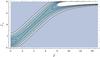 |
Fig. B.1 The posterior Rice distribution using the “projected” prior of Eq. (B.5) with I0/Σ = 8 (a very small value). The distribution of the measured values near the physically-maximum value is notably different than the previous corresponding figures for the Jeffreys and uniform polar prior but the small-value behavior is nearly exact to the Jeffreys case. |
All Tables
Median estimator critical values of p such that Prob(p0 = 0) = 1/2 for the Jeffreys prior.
Median estimator critical values of p such that Prob(p0 = 0) = 1/2 for the uniform polar prior.
All Figures
|
Fig. 1 Contour plots of |
| In the text | |
|
Fig. 2 Two contour plots of the Rice distribution (Eq. (16)). The contours are spaced by 0.1 intervals. The value of
σ is mostly unimportant for
|
| In the text | |
|
Fig. 3 Contour plots of |
| In the text | |
|
Fig. 4 Contour plots of |
| In the text | |
|
Fig. 5 A comparison of “random” points generated with the Jeffreys prior and the uniform polar prior. |
| In the text | |
|
Fig. 6 Two contour plots of the posterior Rice distribution (Eq. (46)) with
|
| In the text | |
|
Fig. 7 Two contour plots of the posterior Rice distribution (Eq. (46)) with
|
| In the text | |
|
Fig. 8 These four panels show the posterior distribution
|
| In the text | |
|
Fig. 9 These four panels show the posterior distribution
|
| In the text | |
|
Fig. 10 This plot compares the classical angle distribution,
G(φ|p0,φ0,σ),
to the Bayesian distribution,
T(φ0|p,φ,σ), with
|
| In the text | |
|
Fig. 11 This plot compares the classical angle distribution,
G(φ|p0,φ0,σ)
(red), to the Bayesian distribution,
T(φ0|p,φ,σ) (blue),
with |
| In the text | |
|
Fig. 12 This figure is a flow chart to help remember the relationships between the distributions presented. “Marg.” stands for marginalization over the accompanying variable. |
| In the text | |
|
Fig. B.1 The posterior Rice distribution using the “projected” prior of Eq. (B.5) with I0/Σ = 8 (a very small value). The distribution of the measured values near the physically-maximum value is notably different than the previous corresponding figures for the Jeffreys and uniform polar prior but the small-value behavior is nearly exact to the Jeffreys case. |
| In the text | |
Current usage metrics show cumulative count of Article Views (full-text article views including HTML views, PDF and ePub downloads, according to the available data) and Abstracts Views on Vision4Press platform.
Data correspond to usage on the plateform after 2015. The current usage metrics is available 48-96 hours after online publication and is updated daily on week days.
Initial download of the metrics may take a while.