| Issue |
A&A
Volume 527, March 2011
|
|
|---|---|---|
| Article Number | A30 | |
| Number of page(s) | 7 | |
| Section | The Sun | |
| DOI | https://doi.org/10.1051/0004-6361/201015491 | |
| Published online | 21 January 2011 | |
Nonlinear force-free field extrapolation in spherical geometry: improved boundary data treatment applied to a SOLIS/VSM vector magnetogram
1
Max-Planck-Institut für Sonnensystemforschung,
Max-Planck-Strasse 2,
37191
Katlenburg-Lindau,
Germany
e-mail: This email address is being protected from spambots. You need JavaScript enabled to view it.
; This email address is being protected from spambots. You need JavaScript enabled to view it.
; This email address is being protected from spambots. You need JavaScript enabled to view it.
2
Addis Ababa University, College of Education, Department of
Physics Education, PO Box
1176, Addis Ababa,
Ethiopia
e-mail: This email address is being protected from spambots. You need JavaScript enabled to view it.
3
National Solar Observatory, Sunspot, NM
88349,
USA
e-mail: This email address is being protected from spambots. You need JavaScript enabled to view it.
Received:
28
July
2010
Accepted:
23
November
2010
Abstract
Context. Understanding the 3D structure of coronal magnetic field is important to understanding: the onset of flares and coronal mass ejections, and the stability of active regions, and to monitoring the magnetic helicity and free magnetic energy and other phenomena in the solar atmosphere. Routine measurements of the solar magnetic field are mainly carried out in the photosphere. Therefore, one has to infer the field strength in the upper layers of the solar atmosphere from the measured photospheric field based on the assumption that the corona is force-free. Meanwhile, those measured data are inconsistent with the above force-free assumption. Therefore, one has to apply some transformations to these data before nonlinear force-free extrapolation codes can be applied.
Aims. Extrapolation codes in Cartesian geometry for modelling the magnetic field in the corona do not take the curvature of the Sun’s surface into account and can only be applied to relatively small areas, e.g., a single active region. Here we apply a method for nonlinear force-free coronal magnetic field modelling and preprocessing of photospheric vector magnetograms in spherical geometry using the optimization procedure.
Methods. We solve the nonlinear force-free field equations by minimizing a functional in spherical coordinates over a restricted area of the Sun. We extend the functional by an additional term, which allows us to incorporate measurement errors and treat regions lacking observational data. We use vector magnetograph data from the Synoptic Optical Long-term Investigations of the Sun survey (SOLIS) to model the coronal magnetic field. We study two neighbouring magnetically connected active regions observed on May 15 2009.
Results. For vector magnetograms with variable measurement precision and randomly scattered data gaps (e.g., SOLIS/VSM), the new code yields field models that satisfy the solenoidal and force-free condition significantly better as it allows deviations between the extrapolated boundary field and observed boundary data within the measurement errors. Data gaps are assigned an infinite error. We extend this new scheme to spherical geometry and apply it for the first time to real data.
Key words: magnetic fields / Sun: corona / Sun: photosphere / methods: numerical
© ESO, 2011
1. Introduction
Observations have shown that physical conditions in the solar atmosphere are strongly
controlled by the solar magnetic field. The magnetic field also provides the link between
different manifestations of solar activity such as, for instance, sunspots, filaments,
flares, or coronal mass ejections. Therefore, the information about the 3D structure of
magnetic field vector throughout the solar atmosphere is crucially important. Routine
measurements of the solar vector magnetic field are mainly carried out in the photosphere.
Therefore, one has to use numerical modelling to infer the field strength into the upper
layers of the solar atmosphere from the measured photospheric field based on the assumption
that the corona is force-free. Owing to the low value of the plasma β (the
ratio of gas pressure to magnetic pressure) (Gary
2001), the solar corona is magnetically dominated. To describe the equilibrium
structure of the coronal magnetic field when non-magnetic forces are negligible, the
force-free assumption is then appropriate:  (1)
(1) (2)
(2) (3)where
B is the magnetic field and
Hobs is the 2D observed surface magnetic field in
the photosphere. Extrapolation methods have been developed for different types of force-free
fields: potential field extrapolation (Schmidt 1964;
Semel 1967), linear force-free field extrapolation
(Chiu & Hilton 1977; Seehafer 1978, 1982; Semel 1988; Clegg et al.
2000), and nonlinear force-free field extrapolation (Sakurai 1981; Wu et al. 1990;
Cuperman et al. 1991; Demoulin et al. 1992; Mikic & McClymont
1994; Roumeliotis 1996; Amari et al. 1997, 1999; Yan & Sakurai 2000; Valori et al. 2005; Wheatland 2004; Wiegelmann 2004; Amari et al. 2006; Inhester & Wiegelmann 2006). Among these, the nonlinear force-free field
has the most realistic description of the coronal magnetic field. For a more complete review
of existing methods for computing nonlinear force-free coronal magnetic fields, we refer to
the review papers by Amari et al. (1997), Schrijver et al. (2006), Metcalf et al. (2008), and Wiegelmann
(2008).
(3)where
B is the magnetic field and
Hobs is the 2D observed surface magnetic field in
the photosphere. Extrapolation methods have been developed for different types of force-free
fields: potential field extrapolation (Schmidt 1964;
Semel 1967), linear force-free field extrapolation
(Chiu & Hilton 1977; Seehafer 1978, 1982; Semel 1988; Clegg et al.
2000), and nonlinear force-free field extrapolation (Sakurai 1981; Wu et al. 1990;
Cuperman et al. 1991; Demoulin et al. 1992; Mikic & McClymont
1994; Roumeliotis 1996; Amari et al. 1997, 1999; Yan & Sakurai 2000; Valori et al. 2005; Wheatland 2004; Wiegelmann 2004; Amari et al. 2006; Inhester & Wiegelmann 2006). Among these, the nonlinear force-free field
has the most realistic description of the coronal magnetic field. For a more complete review
of existing methods for computing nonlinear force-free coronal magnetic fields, we refer to
the review papers by Amari et al. (1997), Schrijver et al. (2006), Metcalf et al. (2008), and Wiegelmann
(2008).
The magnetic field is not force-free in the photosphere, but becomes force-free roughly 400 km above the photosphere (Metcalf et al. 1995). Nonlinear force-free extrapolation codes can be applied only to low plasma-β regions, where the force-free assumption is justified. The preprocessing scheme used until now modifies observed photospheric vector magnetograms with the aim of approximating the magnetic field vector at the bottom of the force-free domain (Wiegelmann et al. 2006; Fuhrmann et al. 2007; Tadesse et al. 2009). The resulting boundary values are expected to be more suitable for an extrapolation into a force-free field than the original values. Preprocessing is important to NLFF-codes that use the magnetic field vector on the boundary directly. Consistent computations for the Grad-Rubin method, which use Bn and Jn (or α) as boundary conditions were carried out by Wheatland & Régnier (2009).
In this paper, we use a larger computational domain that accommodates most of the connectivity within the coronal region. We also take the uncertainties of measurements in vector magnetograms into account as suggested in DeRosa et al. (2009). We implement the preprocessing procedure of Tadesse et al. (2009) to SOLIS data in spherical geometry by considering the curvature of the Sun’s surface within the large field of view containing two active regions. We use a spherical version of the optimization procedure implemented in Cartesian geometry in Wiegelmann & Inhester (2010) for synthetic boundary data.
2. Method
2.1. The SOLIS/VSM instrument
In this study, we use vector magnetogram observations from the Vector Spectromagnetograph (VSM, see Jones et al. 2002), which is part of the Synoptic Optical Long-term Investigations of the Sun (SOLIS) synoptic facility (SOLIS, see Keller et al. 2003). VSM/SOLIS currently operates at the Kitt Peak National Observatory, Arizona, and has provided magnetic field observations of the Sun almost continuously since August 2003.
VSM is a full disk Stokes polarimeter. As part of daily synoptic observations, it takes four different observations in three spectral lines: Stokes I (intensity), V (circular polarization, Q, and U (linear polarization) in photospheric spectral lines FeI630.15 nm and FeI630.25 nm, Stokes I and V in FeI630.15 nm and FeI630.25 nm, similar observations in chromospheric spectral line CaII854.2 nm, and Stokes I in the HeI1083.0 nm line and the near by SiIspectral line. Observations of I, Q, U, and V are used to construct full disk vector magnetograms, while I − V observations are employed to create separate full disk longitudinal magnetograms in the photosphere and the chromosphere.
In this study, we use a vector magnetogram observed on 15 May 2009. The data were taken with 1.125 arcsec pixel size and 2.71 pm spectral sampling. In December 2009, SOLIS/VSM upgraded its cameras from Rockwell (90 Hz, 18 micron pixels) to Sarnoff (300 Hz, 16 micron pixels). This camera upgrade has resulted in improved spatial and spectral sampling. The noise level for a line-of-sight component is about 1 Gauss. However, noise due to atmospheric seeing may be much higher, and the final measurement error depends on the measured flux, its spatial distribution, as well as the seeing conditions. A rough estimate suggests a noise level of a few tens of Gauss for areas with a strong horizontal gradient of magnetic field and about 1 arcsec atmospheric seeing.
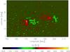 |
Fig.1 Surface contour plot of radial magnetic field vector, and vector field plot of transverse field indicated by black arrows. |
To create a single magnetogram, the solar disk image is scanned from terrestrial south to north; it takes about 20 min to complete one vector magnetogram. After the scan is done, the data are sent to an automatic data reduction pipeline that includes dark and flat field correction. Once the spectra are properly calibrated, full disk vector (magnetic field strength, inclination, and azimuth) magnetograms are created using two different approaches. Quick-look (QL) vector magnetograms are created based on an algorithm by Auer et al. (1977). The algorithm uses the Milne-Eddington model of solar atmosphere, which assumes that the magnetic field is uniform (no gradients) through the layer of spectral line formation (Unno 1956). It also assumes symmetric line profiles, disregards magneto-optical effects (e.g., Faraday rotation), and does not distinguish the contributions of magnetic and non-magnetic components in spectral line profiles (i.e., magnetic filling factor is set to unity). A complete inversion of the spectral data is performed later using a technique developed by Skumanich & Lites (1987). This latter inversion (called ME magnetogram) also employs Milne-Eddington model of atmosphere, but solves for magneto-optical effects and determines the magnetic filling factor i.e., (the fractional contribution of magnetic and non-magnetic components to each pixel). The ME inversion is only performed for pixels with spectral line profiles above the noise level. For pixels below the polarimetric noise threshold, the magnetic field parameters are set to zero.
From the measurements, the azimuths of transverse magnetic field can be determined with 180-degree ambiguity. This ambiguity is resolved using the non-potential field calculation (NPFC, see Georgoulis 2005). The NPFC method was selected on the basis of a comparative investigation of several methods for 180-degree ambiguity resolution (Metcalf et al. 2006). Both QL and ME magnetograms can be used for potential and/or force-free field extrapolation. However, in strong fields inside sunspots, the QL field strengths may exhibit an erroneous decrease inside the sunspot umbra due to so-called magnetic saturation. For this study, we choose to use fully inverted ME magnetograms. Figure 1 shows a map of the radial component of the field as a contour plot with the transverse magnetic field depicted as black arrows. For this particular dataset, about 80% of the data pixels are undetermined and as a result the ratio of data gaps to total number of pixels is large.
2.2. Preprocessing of SOLIS data
The preprocessing scheme of Tadesse et al. (2009)
involves minimizing a two-dimensional functional of quadratic form in spherical geometry
similar to 
 (4)where
H is the preprocessed surface magnetic field from the
input observed field Hobs. Each of the
constraints Ln is weighted by an as yet
undetermined factor μn. The first term
(n = 1) corresponds to the force-balance condition, the next
(n = 2) to the torque-free condition, and the last term
(n = 4) controls the smoothing. The explicit form of
L1, L2, and
L4 can be found in Tadesse
et al. (2009). The term (n = 3) ensures that the optimized
boundary condition agrees with the measured photospheric data. In the case of SOLIS/VSM
data, we modified L3 with respect to the one in Tadesse et al. (2009), to treat those data gaps, to
become
(4)where
H is the preprocessed surface magnetic field from the
input observed field Hobs. Each of the
constraints Ln is weighted by an as yet
undetermined factor μn. The first term
(n = 1) corresponds to the force-balance condition, the next
(n = 2) to the torque-free condition, and the last term
(n = 4) controls the smoothing. The explicit form of
L1, L2, and
L4 can be found in Tadesse
et al. (2009). The term (n = 3) ensures that the optimized
boundary condition agrees with the measured photospheric data. In the case of SOLIS/VSM
data, we modified L3 with respect to the one in Tadesse et al. (2009), to treat those data gaps, to
become  (5)In this integral,
W(θ,φ) = diag(wradial,wtrans,wtrans)
is a diagonal matrix which gives different weights to the different observed surface field
components depending on their relative measurement accuracy. A careful choice of the
preprocessing parameters μn ensures that the
preprocessed magnetic field H does not deviate from the
original observed field Hobs by more than the
measurement errors. As a result of the parameter study in this work, we found that
μ1 = μ2 = 1.0,
μ3 = 0.03, and μ4 = 0.45 as
optimal values.
(5)In this integral,
W(θ,φ) = diag(wradial,wtrans,wtrans)
is a diagonal matrix which gives different weights to the different observed surface field
components depending on their relative measurement accuracy. A careful choice of the
preprocessing parameters μn ensures that the
preprocessed magnetic field H does not deviate from the
original observed field Hobs by more than the
measurement errors. As a result of the parameter study in this work, we found that
μ1 = μ2 = 1.0,
μ3 = 0.03, and μ4 = 0.45 as
optimal values.
2.3. Optimization principle
Equations (1) and (2) can be solved with the help of an
optimization principle, as proposed by Wheatland et al.
(2000) and generalized by Wiegelmann
(2004) for Cartesian geometry. The method minimizes a joint measure of the
normalized Lorentz forces and the divergence of the field throughout the volume of
interest, V. Throughout this minimization, the photospheric boundary of
the model field B is matched exactly to the observed
Hobs and possibly preprocessed magnetogram
values H. Here, we use the optimization approach for
functional (Lω) in spherical geometry (Wiegelmann 2007; Tadesse et al. 2009) along with the new method, which instead of an exact match
enforces a minimal deviation between the photospheric boundary of the model
field B and the magnetogram field
Hobs by adding an appropriate surface
integral term Lphoto (Wiegelmann & Inhester 2010). These terms are given by
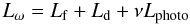 (6)
(6)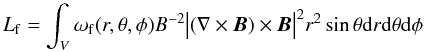
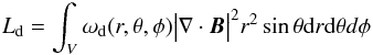
 where
Lf and Ld measure how well the
force-free Eqs. (1) and
divergence-free (2) conditions are
fulfilled, respectively, and both ωf(r,θ,φ)
and ωd(r,θ,φ) are weighting functions. The
third integral, Lphoto, is the surface integral over the
photosphere which allows us to relax the field on the photosphere towards force-free
solution without too much deviation from the original surface field data, and the term
W(θ,φ) is the diagonal matrix
in Eq. (5).
where
Lf and Ld measure how well the
force-free Eqs. (1) and
divergence-free (2) conditions are
fulfilled, respectively, and both ωf(r,θ,φ)
and ωd(r,θ,φ) are weighting functions. The
third integral, Lphoto, is the surface integral over the
photosphere which allows us to relax the field on the photosphere towards force-free
solution without too much deviation from the original surface field data, and the term
W(θ,φ) is the diagonal matrix
in Eq. (5).
Numerical tests of the effect of the new term Lphoto were performed by Wiegelmann & Inhester (2010) in Cartesian geometry for a synthetic magnetic field vector generated from Low & Lou model (Low & Lou 1990). They showed that this new means of incorporating the observed boundary field allows us to cope with data gaps as they appear in SOLIS and other vector magnetogram data. Within this work, we use a spherical geometry for the full disk data from SOLIS. We adopt a spherical grid r, θ, φ with nr, nθ, nφ grid points in the direction of radius, latitude, and longitude, respectively. The method works as follows:
-
We compute an initial source surface potential field in thecomputational domain fromHrobs, the normal component of the surface field at the photosphere at r = 1 R⊙. The computation is performed by assuming that a currentless (J = 0 or ∇ × B = 0) approximation holds between the photosphere and some spherical surface Ss (source surface where the magnetic field vector is assumed radial). We computed the solution of this boundary-value problem in a standard form of harmonic expansion in terms of eigen-solutions of the Laplace equation written in a spherical coordinate system, (r,θ,φ).
-
We minimize Lω (Eqs. (6)) iteratively without constraining Hobs at the photosphere boundary as in a previous version of Wheatland algorithm (Wheatland et al. 2000). The model magnetic field B at the surface is gradually driven towards the observations, while the field in the volume V relaxes to be force-free. If the observed field is inconsistent, the difference B − Hobs or B − H (for preprocessed data) remains finite depending on the control parameter ν. At data gaps in Hobs, we set wradial = 0 and wtrans = 0, and the respective field value is automatically ignored.
-
The state Lω = 0 corresponds to a perfect force-free and divergence-free state and exact agreement of the boundary values B with observations Hobs in regions where wradial and wtrans are greater than zero. For inconsistent boundary data, the force-free and solenoidal conditions can still be fulfilled, but the surface term Lphoto will remain finite. This results in some deviation of the bottom boundary data from the observations, especially in regions where wradial and wtrans are small. The parameter ν is tuned so that these deviations do not exceed the local estimated measurement error.
-
The iteration stops when Lω becomes stationary as ΔLω / Lω < 10-4.
3. Results
We use the vector magnetograph data from the Synoptic Optical Long-term Investigations of the Sun survey (SOLIS) to model the coronal magnetic field. We extrapolate by means of Eq. (6) both the observed field Hobs measured above two active regions observed on May 15 2009 and preprocessed surface field (H obtained from Hobs applying our preprocessing procedure). We compute 3D magnetic field in a wedge-shaped computational box V, which includes an inner physical domain V′ and the buffer zone (the region outside the physical domain), as shown in Fig. 3 of the bottom boundary on the photosphere. The wedge-shaped physical domain V′ has its latitudinal boundaries at θmin = 3° and θmax = 42°, longitudinal boundaries at φmin = 153° and φmax = 212°, and radial boundaries at the photosphere (r = 1 R⊙) and r = 1.75 R⊙.
 |
Fig.2 Left: full disc vector magnetogram of May 15 2009 at 16:02UT. Middle: SOHO/EIT image of the Sun on the same day at 16:00 UT. Right: potential magnetic-field line plot of SOLIS vector magnetogram at 16:02 UT, which has been computed from the observed radial component. |
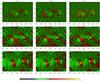 |
Fig.3 Top row: radial surface vector field difference between a) modelled B without preprocessing and Hobs, b) modelled Bpre and Hobs, c) initial potential and Hobs. Middle row: latitudinal surface vector field difference between d) modelled B without preprocessing and Hobs, e) modelled Bpre and Hobs, and f) initial potential and Hobs. Bottom row: longitudinal surface vector field difference between g) modelled B without preprocessing and Hobs, h) modelled Bpre and Hobs, and i) initial potential and Hobs. The vertical and horizontal axes show latitude, θ and longitude, φ in degree on the photosphere respectively. |
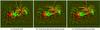 |
Fig.4 a) Some field lines for the potential field reconstruction. b) Nonlinear force-free reconstruction from SOLIS data without preprocessing. c) Nonlinear force-free reconstruction from preprocessed SOLIS data. The panels show the same FOV as in Fig. 2 (right panel). |
The weighting functions ωf and ωd in Lf and Ld in Eq. (6) are chosen to be unity within the inner physical domain V′ and decline with a cosine profile in the buffer boundary region (Wiegelmann 2004; Tadesse et al. 2009). They reach a zero value at the boundary of the outer volume V. The distance between the boundaries of V′ and V is chosen to be nd = 10 grid points wide. The framed region in Figs. 3a − i corresponds to the lower boundary of the physical domain V′ with a resolution of 132 × 196 pixels in the photosphere. The original full disc vector magnetogram has a resolution of 1788 × 1788 pixels out of which we extracted 142 × 206 pixels for the lower boundary of the computational domain V, which corresponds to 550 Mm × 720 Mm on the photosphere.
The main reason for the implementation of the new term Lphoto in Eq. (6) is that we need to work with boundary data of different noise levels and qualities or even neglect some data points completely. SOLIS/VSM provides full-disk vector-magnetograms, but for some individual pixels the inversion from line profiles to field values may not have been successfully inverted and field data there will be missing for these pixels. Since the old code without the Lphoto term requires complete boundary information, it cannot be applied to this set of SOLIS/VSM data. In our new code, these data gaps are treated by setting W = 0 for these pixels in Eq. (6). For those pixels, for which Hobs was successfully inverted, we allow deviations between the model field B and the input fields either observed Hobs or preprocessed surface field H using Eq. (6), so that the model field can be iterated closer to a force-free solution even if the observations are inconsistent. This balance is controlled by the Lagrangian multiplier ν as explained in Wiegelmann & Inhester (2010), where we used wradial = 100wtrans for the surface fields both from data with preprocessing and without.
Figure 2 shows the position of the active region on the solar disk for both the SOLIS full-disk magnetogram1, and the SOHO/EIT image of the Sun observed at 195 Å on the same day at 16:00 UT2. As stated in Sect. 2.3, the potential field is used as the initial condition for iterative minimization required in Eq. (6). The respective potential field is shown in the rightmost panel of Fig. 2. During the iteration, the code forces the photospheric boundary of B towards observed field values Hobs or H (for preprocessed data) and ignores data gaps in the magnetogram. A deviation between surface vector field from model B and either Hobs or H (for preprocessed data) occurs where Hobs is inconsistent with a force-free field. In this sense, the term Lphoto in Eq. (6) acts on Hobs as in the preprocessing, generating a surface field B instead of H from Hobs, which is close to Hobs, but consistent with a force-free field above the surface. In Fig. 3, we therefore compare the difference between the preprocessing procedure and the new extrapolation code (Eq. (6)) on Hobs. The figure shows the surface magnetic field differences of the preprocessed, un-preprocessed, and potential surface fields.
To identify the similarity of vector components on the bottom surface, we calculate their
pixel-wise correlations. The correlation were calculated from  (7)where
vi and
ui are the vectors at each
grid point i on the bottom surface. If the vector fields are identical,
then Cvec = 1; if
vi ⊥ ui,
then Cvec = 0. Table 1
shows the correlations between the surface fields from
Bpre − Hobs,
(where Bpre is the model field obtained from the
preprocessed surface field H using Eq. (6)) and
Bunpre − Hobs,
where Bunpre is the model field the obtained from
observed surface field Hobs using Eq. (6). We computed the vector correlations of the
two surface vector fields for the three components at each grid points to compare how well
they are aligned in each direction. From those values in Table 1, one can see that the preprocessing and extrapolation with Eq. (6) act on
Hobs in a similar way. In Fig. 4, we plot magnetic field lines for the three
configurations in which the vector correlations of potential field lines in the 3D box for
both the extrapolated NLFF with and without preprocessing data are 0.741 and 0.793,
respectively.
(7)where
vi and
ui are the vectors at each
grid point i on the bottom surface. If the vector fields are identical,
then Cvec = 1; if
vi ⊥ ui,
then Cvec = 0. Table 1
shows the correlations between the surface fields from
Bpre − Hobs,
(where Bpre is the model field obtained from the
preprocessed surface field H using Eq. (6)) and
Bunpre − Hobs,
where Bunpre is the model field the obtained from
observed surface field Hobs using Eq. (6). We computed the vector correlations of the
two surface vector fields for the three components at each grid points to compare how well
they are aligned in each direction. From those values in Table 1, one can see that the preprocessing and extrapolation with Eq. (6) act on
Hobs in a similar way. In Fig. 4, we plot magnetic field lines for the three
configurations in which the vector correlations of potential field lines in the 3D box for
both the extrapolated NLFF with and without preprocessing data are 0.741 and 0.793,
respectively.
The correlations between the components of surface fields from (Bpre − Hobs) and (Bunpre − Hobs).
 (8)where
Bpot and Bnlff represent the
potential and NLFF magnetic field, respectively. The free energy is about
5 × 1032 erg. The magnetic energy associated with the potential field
configuration is found to be 32.541 × 1032 erg. Hence,
Enlff exceeds Epot by only 15%.
Table 2 shows the magnetic energy associated with
extrapolated NLFF field configurations with and without preprocessing. The magnetic energy
of the NLFF field configuration obtained from the data without preprocessing is quite higher
than the one from the preprocessed boundary field, as the preprocessing procedure removes
small scale structures.
(8)where
Bpot and Bnlff represent the
potential and NLFF magnetic field, respectively. The free energy is about
5 × 1032 erg. The magnetic energy associated with the potential field
configuration is found to be 32.541 × 1032 erg. Hence,
Enlff exceeds Epot by only 15%.
Table 2 shows the magnetic energy associated with
extrapolated NLFF field configurations with and without preprocessing. The magnetic energy
of the NLFF field configuration obtained from the data without preprocessing is quite higher
than the one from the preprocessed boundary field, as the preprocessing procedure removes
small scale structures.
The magnetic energy associated with extrapolated NLFF field configurations with and without preprocessing.
The electric current density calculated from Ampère’s law, J = ▿ × B / 4π, on the basis of spatially sampled transverse magnetic fields varies widely over an active region. To investigate how errors in the vector magnetograph measurements produce errors in the vertical electric current densities, Liang et al. (2009) numerically simulated the effects of random noise on a standard photospheric magnetic configuration that is produced by electric currents and satisfies the force-free field conditions. Even if the current density can be estimated on the photosphere, it is not intuitively clear how the change in the current density distribution affects a coronal magnetic configuration. Régnier & Priest (2007b) studied these modifications in terms of the geometry of field lines, the storage of magnetic energy, and the amount of magnetic helicity. Figure 5 shows iso-surface plots of current density above the volume of the active region. There are strong current configurations above each active regions. This becomes clear if we compare the total current in-between each active region with the current moving from the left to the right active region. These currents were added up from the surface normal currents emanating from the pixels that are magnetically connected inside or across active regions, respectively. The result is shown in Table 3. The active regions share a decent amount of magnetic flux compared to their internal flux from one polarity to the other. In terms of the electric current, they are much more isolated. The ratio of shared to intrinsic magnetic flux is of the order of unity, while for the electric current those ratios are much less, 1.58 / 49.6 and 1.58 / 32.17, respectively. We can similarly calculate the average value of α on the field lines with the respective magnetic connectivity. The averages are shown in the second row of Table 3. The two active regions are magnetically connected but are much less by electric currents.
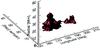 |
Fig.5 Iso-surfaces (ISs) of the absolute current density vector |J| = 100 mA m-2 computed above the active regions. |
The currents and average α calculated from those pixels which are magnetically connected.
4. Conclusion and outlook
We have investigated the coronal magnetic field associated with the AR 11017 on 2009 May 15 and a neighbouring active region by analysing SOLIS/VSM data. We have used the optimization method for the reconstruction of nonlinear force-free coronal magnetic fields in spherical geometry by restricting the code to limited parts of the Sun (Wiegelmann 2007; Tadesse et al. 2009). In contrast to previous implementation, our new code allows us to deal with a lack of data and regions with poor signal-to-noise ratio in the extrapolation in a systematic manner because it produces a field that is closer to a force-free and divergence-free field and tries to match the boundary only where it has been reliably measured (Wiegelmann & Inhester 2010).
For vector magnetograms with a lack of data points and where zero values have been replaced for the signal below a certain threshold value, the new code relaxes the boundary and allows us to fulfill the solenoidal and force-free conditions more reliably as it allows deviations between the extrapolated boundary field and an inconsistent observed boundary data. With the new term, Lphoto extrapolation from Hobs and H yields almost the same 3D field. However, in the latter case the iteration to minimize Eq. (6) saturates in fewer iteration steps. At the same time, preprocessing does not affect the overall configuration of magnetic field and its total energy content.
We plan to use this newly developed code for upcoming data from SDO (Solar Dynamics Observatory)/HMI (Helioseismic and Magnetic Imager) when full disc magnetogram data become available.
Acknowledgments
SOLIS/VSM vector magnetograms are produced cooperatively by NSF/NSO and NASA/LWS. The National Solar Observatory (NSO) is operated by the Association of Universities for Research in Astronomy, Inc., under cooperative agreement with the National Science Foundation. Tilaye Tadesse acknowledges a fellowship of the International Max-Planck Research School at the Max-Planck Institute for Solar System Research and the work of T. Wiegelmann was supported by DLR-grant 50 OC 453 0501.
References
- Amari, T., Aly, J. J., Luciani, J. F., Boulmezaoud, T. Z., & Mikic, Z. 1997, Sol. Phys., 174, 129 [NASA ADS] [CrossRef] [Google Scholar]
- Amari, T., Boulmezaoud, T. Z., & Mikic, Z. 1999, A&A, 350, 1051 [NASA ADS] [Google Scholar]
- Amari, T., Boulmezaoud, T. Z., & Aly, J. J. 2006, A&A, 446, 691 [NASA ADS] [CrossRef] [EDP Sciences] [Google Scholar]
- Auer, L. H., House, L. L., & Heasley, J. N. 1977, Sol. Phys., 55, 47 [NASA ADS] [CrossRef] [Google Scholar]
- Chiu, Y. T., & Hilton, H. H. 1977, ApJ, 212, 873 [NASA ADS] [CrossRef] [Google Scholar]
- Clegg, J. R., Browning, P. K., Laurence, P., Bromage, B. J. I., & Stredulinsky, E. 2000, A&A, 361, 743 [NASA ADS] [Google Scholar]
- Cuperman, S., Demoulin, P., & Semel, M. 1991, A&A, 245, 285 [NASA ADS] [Google Scholar]
- Demoulin, P., Cuperman, S., & Semel, M. 1992, A&A, 263, 351 [NASA ADS] [Google Scholar]
- DeRosa, M. L., Schrijver, C. J., Barnes, G., et al. 2009, ApJ, 696, 1780 [Google Scholar]
- Fuhrmann, M., Seehafer, N., & Valori, G. 2007, A&A, 476, 349 [NASA ADS] [CrossRef] [EDP Sciences] [Google Scholar]
- Gary, G. A. 2001, Sol. Phys., 203, 71 [NASA ADS] [CrossRef] [Google Scholar]
- Georgoulis, M. K. 2005, ApJ, 629, L69 [NASA ADS] [CrossRef] [Google Scholar]
- Inhester, B., & Wiegelmann, T. 2006, Sol. Phys., 235, 201 [NASA ADS] [CrossRef] [Google Scholar]
- Jones, H. P., Harvey, J. W., Henney, C. J., Hill, F., & Keller, U. C. 2002, ESA SP, 505, 15 [Google Scholar]
- Keller, U. C., Harvey, J. W., & Giampapa, M. S. 2003, 4853, 194 [Google Scholar]
- Liang, H. F., Ma, L., Zhao, H. J., & Xiang, F. Y. 2009, New Astron., 14, 294 [NASA ADS] [CrossRef] [Google Scholar]
- Low, B. C., & Lou, Y. Q. 1990, ApJ, 352, 343 [NASA ADS] [CrossRef] [Google Scholar]
- Metcalf, T. R., Jiao, L., McClymont, A. N., Canfield, R. C., & Uitenbroek, H. 1995, ApJ, 439, 474 [NASA ADS] [CrossRef] [Google Scholar]
- Metcalf, T. R., Leka, K. D., Barnes, G., et al. 2006, Sol. Phys., 237, 267 [Google Scholar]
- Metcalf, T. R., Derosa, M. L., Schrijver, C. J., et al. 2008, Sol. Phys., 247, 269 [Google Scholar]
- Mikic, Z., & McClymont, A. N. 1994, in Solar Active Region Evolution: Comparing Models with Observations, ed. K. S. Balasubramaniam & G. W. Simon, ASP Conf. Ser., 68, 225 [Google Scholar]
- Régnier, S., & Priest, E. R. 2007a, ApJ, 669, L53 [NASA ADS] [CrossRef] [Google Scholar]
- Régnier, S., & Priest, E. R. 2007b, A&A, 468, 701 [NASA ADS] [CrossRef] [EDP Sciences] [Google Scholar]
- Roumeliotis, G. 1996, ApJ, 473, 1095 [NASA ADS] [CrossRef] [Google Scholar]
- Sakurai, T. 1981, Sol. Phys., 69, 343 [NASA ADS] [CrossRef] [Google Scholar]
- Schmidt, H. U. 1964, in The Physics of Solar Flares, 107 [Google Scholar]
- Schrijver, C. J., Derosa, M. L., Metcalf, T. R., et al. 2006, Sol. Phys., 235, 161 [Google Scholar]
- Seehafer, N. 1978, Sol. Phys., 58, 215 [NASA ADS] [CrossRef] [Google Scholar]
- Seehafer, N. 1982, Sol. Phys., 81, 69 [NASA ADS] [CrossRef] [Google Scholar]
- Semel, M. 1967, Annales d’Astrophysique, 30, 513 [Google Scholar]
- Semel, M. 1988, A&A, 198, 293 [NASA ADS] [Google Scholar]
- Skumanich, A., & Lites, B. W. 1987, ApJ, 322, 473 [Google Scholar]
- Tadesse, T., Wiegelmann, T., & Inhester, B. 2009, A&A, 508, 421 [NASA ADS] [CrossRef] [EDP Sciences] [Google Scholar]
- Thalmann, J. K., Wiegelmann, T., & Raouafi, N.-E. 2008, A&A, 488, L71 [NASA ADS] [CrossRef] [EDP Sciences] [Google Scholar]
- Unno, W. 1956, Publ. Astron. Soc. Japan, 8, 108 [Google Scholar]
- Valori, G., Kliem, B., & Keppens, R. 2005, A&A, 433, 335 [NASA ADS] [CrossRef] [EDP Sciences] [Google Scholar]
- Wheatland, M. S. 2004, Sol. Phys., 222, 247 [NASA ADS] [CrossRef] [Google Scholar]
- Wheatland, M. S., & Régnier, S. 2009, ApJ, 700, L88 [NASA ADS] [CrossRef] [Google Scholar]
- Wheatland, M. S., Sturrock, P. A., & Roumeliotis, G. 2000, ApJ, 540, 1150 [Google Scholar]
- Wiegelmann, T. 2004, Sol. Phys., 219, 87 [NASA ADS] [CrossRef] [Google Scholar]
- Wiegelmann, T. 2007, Sol. Phys., 240, 227 [NASA ADS] [CrossRef] [Google Scholar]
- Wiegelmann, T. 2008, J. Geophys. Res. (Space Phys.), 113, 3 [Google Scholar]
- Wiegelmann, T., & Inhester, B. 2010, A&A, 516, A107 [NASA ADS] [CrossRef] [EDP Sciences] [Google Scholar]
- Wiegelmann, T., Inhester, B., & Sakurai, T. 2006, Sol. Phys., 233, 215 [NASA ADS] [CrossRef] [Google Scholar]
- Wu, S. T., Sun, M. T., Chang, H. M., Hagyard, M. J., & Gary, G. A. 1990, ApJ, 362, 698 [NASA ADS] [CrossRef] [Google Scholar]
- Yan, Y., & Sakurai, T. 2000, Sol. Phys., 195, 89 [NASA ADS] [CrossRef] [Google Scholar]
All Tables
The correlations between the components of surface fields from (Bpre − Hobs) and (Bunpre − Hobs).
The magnetic energy associated with extrapolated NLFF field configurations with and without preprocessing.
The currents and average α calculated from those pixels which are magnetically connected.
All Figures
|
Fig.1 Surface contour plot of radial magnetic field vector, and vector field plot of transverse field indicated by black arrows. |
| In the text | |
|
Fig.2 Left: full disc vector magnetogram of May 15 2009 at 16:02UT. Middle: SOHO/EIT image of the Sun on the same day at 16:00 UT. Right: potential magnetic-field line plot of SOLIS vector magnetogram at 16:02 UT, which has been computed from the observed radial component. |
| In the text | |
|
Fig.3 Top row: radial surface vector field difference between a) modelled B without preprocessing and Hobs, b) modelled Bpre and Hobs, c) initial potential and Hobs. Middle row: latitudinal surface vector field difference between d) modelled B without preprocessing and Hobs, e) modelled Bpre and Hobs, and f) initial potential and Hobs. Bottom row: longitudinal surface vector field difference between g) modelled B without preprocessing and Hobs, h) modelled Bpre and Hobs, and i) initial potential and Hobs. The vertical and horizontal axes show latitude, θ and longitude, φ in degree on the photosphere respectively. |
| In the text | |
|
Fig.4 a) Some field lines for the potential field reconstruction. b) Nonlinear force-free reconstruction from SOLIS data without preprocessing. c) Nonlinear force-free reconstruction from preprocessed SOLIS data. The panels show the same FOV as in Fig. 2 (right panel). |
| In the text | |
|
Fig.5 Iso-surfaces (ISs) of the absolute current density vector |J| = 100 mA m-2 computed above the active regions. |
| In the text | |
Current usage metrics show cumulative count of Article Views (full-text article views including HTML views, PDF and ePub downloads, according to the available data) and Abstracts Views on Vision4Press platform.
Data correspond to usage on the plateform after 2015. The current usage metrics is available 48-96 hours after online publication and is updated daily on week days.
Initial download of the metrics may take a while.