| Issue |
A&A
Volume 525, January 2011
|
|
|---|---|---|
| Article Number | A108 | |
| Number of page(s) | 13 | |
| Section | Galactic structure, stellar clusters and populations | |
| DOI | https://doi.org/10.1051/0004-6361/201015260 | |
| Published online | 06 December 2010 | |
Searching for Galactic hidden gas through interstellar scintillation: results from a test with the NTT-SOFI detector⋆
1
Laboratoire de l’Accélérateur Linéaire,
IN2P3-CNRS, Université de Paris-Sud,
BP 34,
91898
Orsay Cedex,
France
e-mail: moniez@lal.in2p3.fr
2
Department of Physics, Sharif University of
Technology, PO Box,
11365-9161
Tehran,
Iran
Received:
22
June
2010
Accepted:
17
October
2010
Aims. Stars twinkle because their light propagates through the atmosphere. The same phenomenon is expected at a longer time scale when the light of remote stars crosses an interstellar molecular cloud, but it has never been observed at optical wavelength. In a favorable case, the light of a background star can be subject to stochastic fluctuations on the order of a few percent at a characteristic time scale of a few minutes. Our ultimate aim is to discover or exclude these scintillation effects to estimate the contribution of molecular hydrogen to the Galactic baryonic hidden mass. This feasibility study is a pathfinder toward an observational strategy to search for scintillation, probing the sensitivity of future surveys and estimating the background level.
Methods. We searched for scintillation induced by molecular gas in visible dark nebulae as well as by hypothetical halo clumpuscules of cool molecular hydrogen (H2−He) during two nights. We took long series of 10 s infrared exposures with the ESO-NTT telescope toward stellar populations located behind visible nebulae and toward the Small Magellanic Cloud (SMC). We therefore searched for stars exhibiting stochastic flux variations similar to what is expected from the scintillation effect. According to our simulations of the scintillation process, this search should allow one to detect (stochastic) transverse gradients of column density in cool Galactic molecular clouds of order of ~3 × 10⁻⁵ g/cm2/10 000 km.
Results. We found one light-curve that is compatible with a strong scintillation effect through a turbulent structure characterized by a diffusion radius Rdiff < 100 km in the B68 nebula. Complementary observations are needed to clarify the status of this candidate, and no firm conclusion can be established from this single observation. We can also infer limits on the existence of turbulent dense cores (of number density n > 109 cm-3) within the dark nebulae. Because no candidate is found toward the SMC, we are also able to establish upper limits on the contribution of gas clumpuscules to the Galactic halo mass.
Conclusions. The limits set by this test do not seriously constrain the known models, but we show that the short time-scale monitoring for a few 106 star × hour in the visible band with a >4 m telescope and a fast readout camera should allow one to quantify the contribution of turbulent molecular gas to the Galactic halo. The LSST (Large Synoptic Survey Telescope) is perfectly suited for this search.
Key words: dark matter / Galaxy: disk / Galaxy: halo / Galaxy: structure / local interstellar matter / ISM: molecules
© ESO, 2010
1. Introduction
The present study was made to explore the feasibility of the detection of scintillation effects through nebulae and through hypothetical cool molecular hydrogen (H2 − He) clouds. Considering the results of baryonic compact massive objects searches through microlensing (Tisserand et al. 2007; Wyrzykowski et al. 2010; Alcock et al. 2000; see also the review of Moniez 2010), these clouds should now be seriously considered as a possible major component of the Galactic hidden matter. It has been suggested that a hierarchical structure of cold H2 could fill the Galactic thick disk (Pfenniger et al. 1994; Pfenniger & Combes 1994) or halo (De Paolis et al. 1995; De Paolis et al. 1998), providing a solution for the Galactic hidden matter problem. This gas should form transparent “clumpuscules” of ~30 AU size, with an average density of 109 − 10 cm-3, an average column density of 1024 − 25 cm-2, and a surface filling factor of ~1%. The detection of these structures thanks to the scintillation of background stars would have a major impact on the Galactic dark matter question.
The OSER project (optical scintillation by extraterrestrial refractors) is proposed to search for scintillation of extra-galactic sources through these Galactic – disk or halo – transparent H2 clouds. This project should allow one to detect (stochastic) transverse gradients of column density in cool Galactic molecular clouds on the order of ~3 × 10⁻⁵ g/cm2/10 000 km. The technique can also be used for the nebulae science. The discovery of scintillation through visible nebulae should indeed open a new window to investigate their structure.
The feasibility study described here concerns the search for scintillation through known dark nebulae such as B68 (also identified as LDN57), cb131 (also identified as B93 and L328), through a nebula within the Circinus complex (hereafter called Circinus nebula), and also includes a test for hidden matter search toward the SMC. As discussed below, we did not think it very likely to discover a signal, and the main purpose of the test was to predict the sensitivity of a future optical survey from the measurement of the signal sensitivity in infrared and from the estimate of the variable star background level.
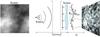 |
Fig. 1 Left: a 2D stochastic phase screen (gray scale) from a simulation of gas affected by Kolmogorov-type turbulence. Right: the illumination pattern from a point source (left) after crossing such a phase screen. The distorted wavefront produces structures at scales of ~Rdiff(λ) and Rref(λ) on the observer’s plane. |
2. The scintillation process
2.1. Basics
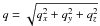
Refraction through an inhomogeneous transparent cloud (hereafter called screen), which is described by a 2D phase delay function φ(x,y) in the plane transverse to the line of sight, distorts the wave-front of incident electromagnetic waves (Fig. 1; Moniez 2003). The luminous amplitude in the observer’s plane after propagation is described by the Huygens-Fresnel diffraction theory. For a point-like, monochromatic source, the intensity in the observer’s plane is affected by interferences which take on the speckle aspect in the case of stochastic inhomogeneities. At least two distance scales characterize this speckle, which are related to the wavelength λ, to the distance of the screen z0, and to the statistical characteristics of the stochastic phase delay function φ:
-
The diffusion radius Rdiff(λ) of the screen, defined as the separation in the screen transverse plane for which the root mean square of the phase delay difference at wavelength λ is 1 radian (Narayan 1992). Formally, Rdiff(λ) is given in a way that ⟨ (φ(x′ + x,y′ + y) − φ(x′,y′))2 ⟩ = 1 where (x′,y′) spans the entire screen plane and (x,y) satisfies
 . The diffusion
radius characterizes the structuration of the inhomogeneities of the cloud, which
are related to the turbulence. As demonstrated in Appendix A, assuming that the
cloud turbulence is isotropic and is described by the Kolmogorov theory up to the
largest scale (the cloud’s width Lz),
Rdiff can be expressed as
. The diffusion
radius characterizes the structuration of the inhomogeneities of the cloud, which
are related to the turbulence. As demonstrated in Appendix A, assuming that the
cloud turbulence is isotropic and is described by the Kolmogorov theory up to the
largest scale (the cloud’s width Lz),
Rdiff can be expressed as ![\begin{equation} R_{\rm diff}(\lambda)=263\, {\rm km} \times \left[\frac{\lambda}{1~\mu{\rm m}}\right]^{\frac{6}{5}} \left[\frac{L_z}{10\,{\rm AU}}\right]^{-\frac{1}{5}} \left[\frac{\sigma_{3n}}{10^{9}\,{\rm cm}^{-3}}\right]^{-\frac{6}{5}}\!\! , \label{expression-rdiff} \end{equation}](/articles/aa/full_html/2011/01/aa15260-10/aa15260-10-eq26.png) (1)where
σ3n is the molecular number density
dispersion within the cloud. In this expression, we assume that the average
polarizability of the molecules in the medium is
α = 0.720 × 10⁻²⁴ cm3, corresponding to a
mixing of 76% of H2 and 24% of He by mass.
(1)where
σ3n is the molecular number density
dispersion within the cloud. In this expression, we assume that the average
polarizability of the molecules in the medium is
α = 0.720 × 10⁻²⁴ cm3, corresponding to a
mixing of 76% of H2 and 24% of He by mass. 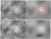
Fig. 2 Simulated illumination map at λ = 2.16 μm on Earth from a point source (up-left)- and from a K0V star (rs = 0.85 R⊙, MV = 5.9) at z1 = 8 kpc (right). The refracting cloud is assumed to be at z0 = 160 pc with a turbulence parameter Rdiff(2.16 μm) = 150 km. The circle shows the projection of the stellar disk (with radius RS = rs × z0/z1). The bottom maps are illuminations in the Ks wide band (λcentral = 2.162 μm, Δλ = 0.275 μm).
-
The refraction radius
![\begin{equation} \label{Rref} R_{\rm ref}(\lambda)\!=\!\frac{\lambda z_0}{R_{\rm diff}}\! \sim\! 30\,860\,{\rm km}\left[\frac{\lambda}{1~\mu{\rm m}}\right]\left[\frac{z_0}{1\,{\rm kpc}}\right]\left[\frac{R_{\rm diff}(\lambda)}{1000\,{\rm km}}\right]^{-1}\!, \end{equation}](/articles/aa/full_html/2011/01/aa15260-10/aa15260-10-eq43.png) (2)is the size in the
observer’s plane of the diffraction spot from a patch of
Rdiff(λ) in the screen’s plane.
(2)is the size in the
observer’s plane of the diffraction spot from a patch of
Rdiff(λ) in the screen’s plane. -
In addition, long scale structures of the screen can possibly induce local focusing/defocusing configurations that produce long time-scale intensity variations.
2.2. Expectations from simulation: intensity modulation, time scale
After crossing an inhomogeneous cloud described by the Kolmogorov turbulence law (Fig. 1, left), the light from a monochromatic point source produces an illumination pattern on Earth made of speckles of a size Rdiff(λ) within larger structures of a size Rref(λ) (see Fig. 2, up-left). The illumination pattern from a real stellar source of radius rs is the convolution of the point-like intensity pattern with the projected intensity profile of the source (projected radius RS = rs × z0/z1) (Fig. 2, up-right). RS is then another characteristic spatial scale that affects the illumination pattern from a stellar (not point-like) source.
We simulated these illumination patterns that are caused by the diffusion of stellar source light through various turbulent media as follows:
-
we first simulated 2D turbulent screens as stochastic phase delay functions Φ(x,y), according to the Kolmogorov law1; series of screens were generated at z0 = 125 pc with 100 km < Rdiff < 350 km;
-
we then computed the expected illumination patterns at λ = 2.162 μm (central wavelength for Ks filter) from diffused background point-like monochromatic sources located at z1 = 1 kpc using the Fast Fourier Transform (FFT) technique (see Fig. 2 up-left). Illumination patterns for other wavelengths and geometrical configurations were deduced by simple scaling. In particular, configurations compatible with the structure of the H2 clumpuscules of (Pfenniger et al. 1994) were produced for the J passband (Rdiff(1.25 μm) ≳ 17 km, corresponding to clumpuscules with Lz = 30 AU and σ3n < nmax = 1010 cm-3);
-
we derived series of patterns from diffused extended stellar sources (radii 0.25 R⊙ < rs < 1.5 R⊙) by convolution (Fig. 2 top-right);
-
finally, we co-added the patterns obtained for the central and the two extreme wavelengths of the Ks (Δλ = 0.275 μm) and J (Δλ = 0.290 μm) passbands to simulate the diffusion of a wide-band source (Fig. 2 down-right).
More details on this simulation will be published in a forthcoming paper (Habibi et al., in prep.).
2.2.1. Modulation
In general, the small speckle from a point-source is almost completely smoothed after
the convolution by the projected stellar profile, and only the large structures of the
size Rref(λ) – or larger – produce a
significant modulation. Therefore, as a result of the spatial coherence limitations, the
modulation of the illumination pattern critically depends on the angular size of the
stellar source
θs = rs/(z0 + z1) ~ rs/z1.
Our Monte-Carlo studies show that the intensity modulation index
 decreases when the ratio of the projected stellar disk RS to
the refraction scale Rref(λ) increases, as
shown in Fig. 3. This ratio can be expressed as
decreases when the ratio of the projected stellar disk RS to
the refraction scale Rref(λ) increases, as
shown in Fig. 3. This ratio can be expressed as
![\begin{equation} \frac{R_{\rm S}}{R_{\rm ref}(\lambda)}\! =\! \frac{r_{\rm s} R_{\rm diff}(\lambda)}{\lambda z_1}\! \sim \! 2.25\left[\frac{\lambda}{1~\mu{\rm m}}\right]^{-1}\!\! \left[\!\frac{r_{\rm s}/z_1}{R_{\odot}/10\,{\rm kpc}}\!\right] \left[\frac{R_{\rm diff}(\lambda)}{1000\,{\rm km}}\right]\cdot \label{contparam} \end{equation}](/articles/aa/full_html/2011/01/aa15260-10/aa15260-10-eq60.png) (3)At the first order, as
intuitively expected, the modulation index only depends on this ratio
RS/Rref(λ)
and not on other parameters of the phase screen or explicitly on λ.
Indeed, the dispersion of mscint for series of
different configurations generated with the same
RS/Rref ratio is compatible
with the statistical dispersion of mscint in series of 10
patterns generated with identical configurations. We empirically found
that the modulation indices plotted as a function of
RS/Rref are essentially
contained between the curves represented by functions
Fmin(x) = 0.17e − 1.2RS/Rref
and
Fmax(x) = 0.2e − 0.95RS/Rref
in Fig. 3.
(3)At the first order, as
intuitively expected, the modulation index only depends on this ratio
RS/Rref(λ)
and not on other parameters of the phase screen or explicitly on λ.
Indeed, the dispersion of mscint for series of
different configurations generated with the same
RS/Rref ratio is compatible
with the statistical dispersion of mscint in series of 10
patterns generated with identical configurations. We empirically found
that the modulation indices plotted as a function of
RS/Rref are essentially
contained between the curves represented by functions
Fmin(x) = 0.17e − 1.2RS/Rref
and
Fmax(x) = 0.2e − 0.95RS/Rref
in Fig. 3.
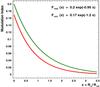 |
Fig. 3 Expected intensity modulation index |
2.2.2. Time scale
Because the 2D illumination pattern sweeps the Earth with a constant speed, simulated
light-curves of scintillating stars have been obtained by regularly sampling the 2D
illumination patterns along straight lines. For a cloud moving with a transverse
velocity VT with respect to the line of sight, the velocity
of the illumination pattern on the Earth is
VT(z0 + z1)/z1 ~ VT
as z0 ≪ z1; neglecting the inner
cloud evolution – as in radio astronomy (frozen screen approximation (Lyne & Graham-Smith 1998) – the flux
variation at a given position is caused by this translation, which induces intensity
fluctuations with a characteristic time scale of
![\begin{eqnarray} t_{\rm ref}(\lambda)&=&\frac{R_{\rm ref}(\lambda)}{V_{\rm T}} \\ &\sim & \!\! 5.2\, \min\left[\frac{\lambda}{1~\mu{\rm m}}\right]\left[\frac{z_0}{1\,{\rm kpc}}\right]\left[\frac{R_{\rm diff}(\lambda)}{1000\,{\rm km}}\right]^{-1}\left[\frac{V_{\rm T}}{100\,{\rm km\,s^{-1}}}\right]^{-1}\!\!\!\! \cdot \nonumber \end{eqnarray}](/articles/aa/full_html/2011/01/aa15260-10/aa15260-10-eq73.png) (4)Therefore
we expect the scintillation signal to be a stochastic fluctuation of the light-curve
with a frequency spectrum peaked around
1/tref(λ) on the order of
(min)-1.
(4)Therefore
we expect the scintillation signal to be a stochastic fluctuation of the light-curve
with a frequency spectrum peaked around
1/tref(λ) on the order of
(min)-1.
As an example, the scintillation at λ = 0.5 μm of a
LMC-star through a Galactic H2 − He cloud located at 10 kpc is characterized
by parameter
RS/Rref(0.5 μm) ~ (rs/R⊙) × (Rdiff(0.5 μm)/222 km).
According to Fig. 3, one expects
 if
x = RS/Rref ≲ 2.4
(
if
x = RS/Rref ≲ 2.4
( ).
This will be the case for LMC (or SMC) stars smaller than the Sun as soon as
Rdiff(0.5 μm) ≲ 530 km. If the
transverse speed of the Galactic cloud is
VT = 200 km s-1, the characteristic
scintillation time scale will be tref ≳ 24 min.
).
This will be the case for LMC (or SMC) stars smaller than the Sun as soon as
Rdiff(0.5 μm) ≲ 530 km. If the
transverse speed of the Galactic cloud is
VT = 200 km s-1, the characteristic
scintillation time scale will be tref ≳ 24 min.
2.3. Some specificities of the scintillation process
In the subsections below we briefly describe the properties and specificities of the scintillation signal that should be used to distinguish a population of scintillating stars from the population of ordinary variable objects.
2.3.1. Chromaticity effect
Because Rref depends on λ, one expects a variation of the characteristic time scale tref(λ) between the red side of the optical spectrum and the blue side. This property is probably one of the best signatures of the scintillation, because it points to a propagation effect, which is incompatible with any type of intrinsic source variability.
2.3.2. Relation between the stellar radius and the modulation index
As shown in Fig. 3, big stars scintillate less than small stars through the same gaseous structure. This characteristic signs the limitations from the spatial coherence of the source and can also be used to statistically distinguish the scintillating population from other variable stars.
2.3.3. Location
Because the line of sight of a scintillating star has to pass through a gaseous structure, we expect the probability for scintillation to be correlated with the foreground – visible gas column-density. Regarding the invisible gas, it may induce clusters of neighboring scintillating stars among a spatially uniform stellar distribution because of foreground – undetected gas structures. This clustering without apparent cause is not expected from other categories of variable stars.
2.4. Foreground effects, background to the signal
Conveniently, atmospheric intensity scintillation is negligible through a large telescope (matm ≪ 1% for a >1 m diameter telescope, Dravins et al. 1997, 1998). Any other atmospheric effect such as absorption variations at the minute scale (because of fast moving cirruses for example) should be easy to recognize as long as nearby stars are monitored together. Asteroseismology, granularity of the stellar surface, spots or eruptions produce variations of very different amplitudes and time scales. A few types of rare recurrent variable stars exhibit emission variations at the minute scale (Sterken & Jaschek 1996), but they could be identified from their spectrum or type. Scintillation should also not be confused with absorption variations caused by the dust distribution in the cloud; indeed, the relative column density fluctuations needed to produce measurable absorption variations (~1%) is higher by several orders of magnitudes than the fluctuations that are able to produce a significant scintillation (only a few 10-7 for the clumpuscules, and 10-3 for the Bok globules within a domain of Rdiff size).
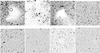 |
Fig. 4 The four monitored fields, showing the structures of the nebulae and the background stellar densities. From left to right: B68, Circinus, cb131, and the SMC. Up: images from the ESO-DSS2 in R. Down: our corresponding template images (in Ks for B68, cb131 and Circinus, in J for SMC). North is up and East is left. The circles on the B68 images show the position of our selected candidate. |
Observations and data reduction results.
2.5. Expected optical depth
Assuming a Galactic halo completely made of clumpuscules of mass Mc = 10-3 M⊙, their sky coverage (geometrical optical depth) toward the LMC or the SMC should be on the order of 1% according to Pfenniger et al. (1994). This calculation agrees with a simple estimate based on the density of the standard halo model taken from (Caldwell & Coulson 1986). Here, we are considering only those structures that can be detected through scintillation. Therefore we quantify the sky coverage of the turbulent sub-structures that can produce this scintillation. We define the scintillation optical depth τλ(Rdiff max) as the probability for a line of sight to cross a gaseous cloud with a diffusion radius (at λ) Rdiff(λ) < Rdiff max; this optical depth is lower than (or equal to) the total sky coverage of the clumpuscules, because it takes into account only those gaseous structures with a minimum turbulence strength; if Rdiff → ∞, all gaseous structures account for the optical depth and τλ(∞) is the total sky coverage of the clumpuscules.
3. Feasibility studies with the NTT
As shown in Fig. 3, the search for scintillation induced by transparent Galactic molecular clouds makes it necessary to sample at the sub-minute scale the luminosity of LMC or SMC main sequence stars with a photometric precision of – or better – than ~1%. In principle, this can be achieved with a two meter class telescope with a high quantum efficiency detector and a short dead-time between exposures. To test the concept in a somewhat controlled situation, we also decided to search for scintillation induced by known gas through visible nebulae.
We found that the only setup available for this short time-scale search was the ESO NTT-SOFI combination in the infrared, with the additional benefit to enable the monitoring of optically obscured stars that are located behind dark nebulae. The drawback is that observations in infrared do not benefit from the maximum of the stellar emission and the 3.6 m diameter telescope is barely sufficient to achieve the required photometric precision.
3.1. The targets
Considering the likely low optical depth of the scintillation process, all our fields were selected to contain large numbers of target stars. This criterion limited our search to the Galactic plane and to the LMC and SMC fields. For the search through visible nebulae (in the Galactic plane) we added the following requirements:
-
maximize the gas column density to benefit from a long phase delay. Data from 2MASS (Skrutskie et al. 2006) where used to select the clouds that induce the stronger reddening of background stars, pointing toward the thickest clouds;
-
we selected nebulae that are strongly structured (from visual inspection) and favored those with small spatial scale structures;
-
we chose fields that contain a significant fraction of stars that are not behind the nebula to be used as a control sample.
We decided to observe toward the nebulae with the Ks filter to allow the monitoring of highly extincted stars (i.e. behind a high gas column density).
To make a test search for transparent (hidden) gas, we selected a crowded field in the SMC (LMC was not observable at the time of observations). Then we used the J filter to collect the maximum light fluxes attainable with the SOFI detector. Figure 4 shows the four monitored (4.92 × 4.92) arcmin2 size fields in R and in the Ks or J passbands; Table 1 gives their list and characteristics and also the main observational and analysis information.
Through the cores of B68 and Circinus, gas column densities of ~1022 atoms/cm2 induce an average phase delay of 250 × 2π at Ks central wavelength (λ = 2.16 μm). According to our studies, a few percent scintillation signal is expected from stars smaller than the Sun if relative column density fluctuations of only ~10-3 occur within less than a few thousand kilometers (corresponding to Rdiff ≲ 2000 km). These fluctuations – which are probably rare – could induce dust absorption variations of only ~10-3, which can be neglected. The expected time scale of the scintillation would be tref ≳ 5 min, assuming VT ~ 20 km s-1.
3.2. The observations
During two nights of June 2006 we took a total of 4749 consecutive exposures of Texp = 10 s, with the infra-red 1024 × 1024 pixel SOFI detector in Ks (λ = 2.16 μm) toward B68, Circinus, cb131, and in J (λ = 1.25 μm) toward the SMC (see Table 1 for details). We recall that for a dedicated search for transparent hidden matter, measuring visible light (B, V, R or G filters) – corresponding to the maximum stellar emission – would be better.
4. Data reduction
4.1. Photometric reduction
With the EROS software (Ansari 1996) we produced the light-curves φ(t) of a few thousands of stars for each target. The reference catalogs of the monitored stars where established from templates obtained through the standard GASGANO procedure (ESO 2001) by co-adding 10 exposures of 60s each for the B68, Circinus, and cb131 fields (13 exposures for the SMC field). The photometric measurements were all aligned with respect to these templates. We experimented with several techniques for the photometric reduction (aperture photometry and Gaussian point spread function (PSF) fitting). We found that the most precise photometric technique, which provides the smallest average point-to-point variation, is the Gaussian PSF fitting. We observed that the Gaussian fit quality of the PSF decreases when the seeing (i.e. the width of the PSF) is small. This effect induces some correlation between the seeing and the estimated flux, and we systematically corrected the flux for this effect, according to a procedure described in Tisserand (2004). Figure 5 shows the dispersion of the measurements along the light-curves. This dispersion depends on the photometric precision and on the – possible but rare – intrinsic stellar apparent variability. We checked that it is not affected by the dust by considering separately a control sample of stars (Fig. 7) that are apart from the nebula (Fig. 5, upper panel). We interpret the lower envelope of Fig. 5 as the best photometric precision achieved on (stable) stars at a given magnitude. The outliers that are far above this envelope can be caused by a degradation of the photometric precision in a crowded environment, by the parasitic effect of bad pixels, or by a real variation of the incoming flux. The best photometric precision does not simply result from the Poissonian fluctuations of the numbers of photoelectrons Nγe. We discuss the main sources of the precision limitation in Appendix B.
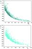 |
Fig. 5 Dispersion of the photometric measurements along the light-curves as a function of the mean Ks magnitude (up) and J magnitude (down). Each dot corresponds to one light-curve. In the upper panel, the small black dots correspond to control stars that are not behind the gas; the big blue dots correspond to stars located behind the gas; the big star marker indicates our selected candidate. |
4.2. Calibration
The photometric calibration was done using the stars from the 2MASS catalog in our fields (Skrutskie et al. 2006). These stars were found only in the SMC and B68 fields. Because all our fields were observed during the same nights with stable atmospheric conditions, we extrapolated the calibration in the Ks band from B68 to cb131 and Circinus, after checking on series of airmass-distributed images that the airmass differences between the reference images (which are smaller that 0.1) could not induce flux variations higher than 0.1 mag.
5. Analysis
5.1. Filtering
We removed the lowest quality images, stars, and mearurements by requiring the following criteria.
-
Fiducial cuts: we do not measure the luminosity of objects closer than 100 pixels from the limits of the detector to avoid visible defects on its borderlines. The effective size of the monitored fields is then 4.44 × 4.44 arcmin2.
We remove the images with poor reconstructed seeing by requiring
 ,
where
,
where  and σs are the mean and rms of the seeing distributions
(see Fig. 6).
and σs are the mean and rms of the seeing distributions
(see Fig. 6). 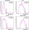
Fig. 6 Seeing distributions of the images towards the four targets. The images with larger seeing than the position of the arrow are discarded.
-
We remove the images with an elongated PSF that have an eccentricity e > 0.55.
-
We reject the measurements with a poor PSF fit quality. This quality varies with the seeing, the filter, the position of the object on the detector, and also with the flux of the star. We require the χ2 of the fit to satisfy χ2/d.o.f. < 4.
-
Minimum flux: we keep only stars with an instrumental flux φ > 1000 ADU (corresponding to J < 17.8, Ks < 17.1) to allow a reproducibility of the photometric measurements better than ~15% in Ks and ~8% in J. The number of these stars are given in Table 1.
-
We require at least 10 good quality measurements per night per light-curve before searching for variabilities.
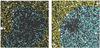 |
Fig. 7 Definition of the control regions (yellow dots) and the search regions (blue dots) toward B68 (left) and cb131 (right). |
5.2. Selecting the most variable light-curves
We expect the scintillation signal to produce a stochastic fluctuation of the incoming
flux with a frequency spectrum peaked around
1/tref(λ), on the order of
(min)-1. The point-to-point variations of a stellar light-curve are caused by
the photometric uncertainties (statistical and systematical) and by the possible intrinsic
incoming flux fluctuations. Note that fluctuations with time scales shorter than the
sampling
(δt ≲ ti + 1 − ti ~ 15 s)
are smoothed in our data, and their high-frequency component cannot be detected. To select
a sub-sample that includes the intrinsically most variable objects, we used a simple
criterion – not specific to a variability type –, which allowed us to both check our
ability to detect known variable objects and explore new time domains of variability. Our
criterion is based on the ratio
R = σφ/σint
of the light-curve dispersion σφ to the
“internal” dispersion σint, defined as the rms of the
differences between the flux measurements and the interpolated values from the previous
and next measurements: ![\begin{eqnarray} &&\!\!\!\!\! \sigma_{\rm int} = \\ &&\!\!\!\!\!\sqrt{\frac{1}{N_{\rm meas}}\sum_i \left[ \phi(t_i)\! - \left(\phi(t_{i-1})+[\phi(t_{i+1})\! -\! \phi(t_{i-1})] \frac{t_{i}-t_{i-1}}{t_{i+1}-t_{i-1}}\right)\right]^2 } , \nonumber \end{eqnarray}](/articles/aa/full_html/2011/01/aa15260-10/aa15260-10-eq147.png) (5)where
Nmeas is the number of flux measurements and
φ(ti) is the measured flux
at time ti (the typical
ti − ti − 1
interval is ~15 s). σint quantifies the
point-to-point fluctuations, whereas σφ is
the global dispersion of a light-curve. R is high as soon as there is a
correlation between consecutive fluctuations, either because of incoming flux variations
or systematic effects. Figure 8 shows the
distributions of R versus the apparent magnitude
Ks (J for SMC).
(5)where
Nmeas is the number of flux measurements and
φ(ti) is the measured flux
at time ti (the typical
ti − ti − 1
interval is ~15 s). σint quantifies the
point-to-point fluctuations, whereas σφ is
the global dispersion of a light-curve. R is high as soon as there is a
correlation between consecutive fluctuations, either because of incoming flux variations
or systematic effects. Figure 8 shows the
distributions of R versus the apparent magnitude
Ks (J for SMC).
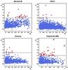 |
Fig. 8 The R = σφ/σint versus Ks (or J) distributions of the light-curves of the monitored stars. The red dots correspond to the most variable light-curves. The green stars indicate two known variable objects toward SMC and our selected candidate toward B68. |
By selecting light-curves with R > 1.6 (in Ks) or R > 1.4 (in J) – the red dots in Fig. 8 – we retain those with a global variation over the two nights that is significantly larger than the point-to-point variations. Because we found that R almost never exceeds the selection threshold in large series of simulated uniform light-curves affected by Gaussian errors, we systematically inspected each of the high R objects. We found that almost all of them are artifacts (all the red dots in Fig. 8); we identified the following causes, which are related to the observational conditions:
-
during the meridian transit of B68, the light-curves of a series of bright stars located in two regions showed an abrupt flux transition, correlated with the equilibrium change in the mechanics of the telescope;
some stars looked temporarily brighter because of contamination from the rotating egrets of bright stars;
we also identified a few stars transiting near hot or dead pixels, which induced a distorsion of the flux determination.
5.3. Sensitivity of the analysis to the known variable objects
Our selection using variable R = σφ/σint is supposed to retain any type of variability as soon as variations occur on a time scale longer than our sampling time. This allowed us to control our sensitivity to known variable stars. This control has been possible only toward the SMC because it is the only field where we found cataloged variable objects. Indeed the CDS and EROS cataloges (Tisserand et al. 2007) contain three variable objects within our SMC-field. We were able to identify two cepheids, HV1562 (, J2000, J = 14.7, periodicity 4.3882 days) and the EROS cepheid (, J2000, J = 16.03, periodicity 2.13581 days). Figure 9 shows the corresponding folded light-curves from the EROS SMC database (phase diagram) (Tisserand et al. 2007; Hamadache et al. 2006; Rahal et al. 2009), on which we superimpose our own observations.
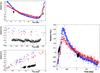 |
Fig. 9 EROS folded light-curves of cepheids HV1562 (upper-left) and of the EROS object () (right) in BEROS and REROS passbands, with our NTT observations in J (black dots). The lower-left panels show details around our observations. |
We are content to note that the light-curves of both objects were successfully selected by our analysis; they correspond to the objects marked by a star in Fig. 8 (SMC). Our precision was sufficient to clearly observe the rapidly ascending phase of HV1562 during night 2, as can be seen in Fig. 9.
The third variable object in the SMC field is OGLE SMC-SC6 148139 (, J2000, B = 16.5). It is a detached eclipsing binary with a periodicity of 1.88508 days. Because no eclipse occured during the data taking, this object was – logically – not selected as a variable by our analysis.
5.4. Signal?
Only one variable object remains toward B68 after removing all artifacts (see Fig. 10 and see its location (J2000) in Fig. 4 left). The star has magnitudes
Ks = 16.6 and J = 20.4; its light is
absorbed by dust by AK = 0.99 magnitude; it
is a main sequence star with possible type ranging from A0 at 9.6 kpc
(rs = 2.4 R⊙) to A5 at 6.1 kpc
(rs = 1.7 R⊙) or from F0 at
5.0 kpc (rs = 1.6 R⊙) to F5 at
4.0 kpc (rs = 1.4 R⊙).
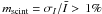
Consequently, it is a star small enough to experience observable scintillation. The
modulation index of the light-curve is m = 0.17, which is quite high but
not incompatible with a variation owing to scintillation. If we consider that this
modulation is caused by a scintillation effect, then it is induced by a turbulent
structure with
RS/Rref < 0.25, according
to Fig. 3; as we know that
rs/z1 > 2.5 R⊙/10 kpc,
we directly conclude from expression (3)
that Rdiff(2.16 μm) < 96 km; using
expression (1), this gives the following
constraint on the size and the density fluctuations of the hypothetic turbulent structure:
![\begin{equation} \sigma_{3n}>1.45\times 10^9 ~{\rm cm}^{-3} \left[\frac{L_z}{17\,000\, \rm AU}\right]^{-\frac{1}{6}}\cdot \end{equation}](/articles/aa/full_html/2011/01/aa15260-10/aa15260-10-eq177.png) (6)The largest possible
outer scale Lz corresponds here to the minor
axis of B68 (17 000 AU), but smaller turbulent structures within the global system may
also happen.
(6)The largest possible
outer scale Lz corresponds here to the minor
axis of B68 (17 000 AU), but smaller turbulent structures within the global system may
also happen.
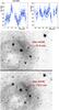 |
Fig. 10 Light-curves for the two nights of observation (top) and images of the selected candidate toward B68 during a low-luminosity phase (middle) and a high-luminosity phase (bottom); North is up, East is left. |
A definitive conclusion on this candidate would need complementary multi-epoch and multicolor observations, as explained in Sect. 2.3.1; but the hypothetic turbulent structure that is possibly responsible for scintillation has probably moved from the line of sight since the time of observations, considering its typical size. Nevertheless, reobserving this object would allow one to check for any other type of variability. Considering the short time scale and the large amplitude fluctuations, a flaring or eruptive star may be suspected, but probably not a spotted star or an effect of astroseismology.
An important result comes from the rarity of these fluctuating objects: there is no significant population of variable stars that can mimic scintillation effects, and future searches should not be overwhelmed by background of fakes.
Ideally, for future observation programs aiming for an unambiguous signature, complementary multiband observations should be planned shortly after the detection of a scintillation candidate. After detection of several candidates, one should also further investigate the correlation between the modulation index and the estimated gas column density to reinforce the scintillation case (see Sects. 2.3.2 and 2.3.3).
6. Establishing limits on the diffusion radius
In the following sections we will establish upper limits on the existence of turbulent gas bubbles based on the observed light-curve modulations. The general technique consists to find the minimum diffusion radius Rdiff for each monitored star that is compatible with the observed modulation.
The smallest diffusion radius compatible with observed stellar light-curve fluctuations
Let us consider a star with radius rs, placed at distance
z1 behind a screen located at z0
(with a projected radius
RS = rs × z0/z1).
If a turbulent structure characterized by Rdiff (with the
corresponding Rref given by Eq. (2)) induces scintillation of the light of this star, the corresponding
modulation mscint is within the limits  (7)as predicted from
Fig. 3.
(7)as predicted from
Fig. 3.
Below we assume that our time sampling is sufficient to take into account any real
variation within a time scale longer than a minute. Then, because the observed modulation
m of a stellar light-curve results from the photometric uncertainties and
from the hypothetic intensity modulation mscint, one can infer
that mscint ≤ m. This inequality combined with
inequality (7) leads to
Fmin(RS/Rref) < m.
Because Fmin is a decreasing function, it follows that
 . Using
Eq. (3) and inverting function
Fmin(x) = 0.17e−1.2x,
this can be expressed as a constraint on the value of Rdiff for
the gas crossed by the light:
. Using
Eq. (3) and inverting function
Fmin(x) = 0.17e−1.2x,
this can be expressed as a constraint on the value of Rdiff for
the gas crossed by the light: ![\begin{equation} R_{\rm diff} > R_{\rm diff}^{\rm min} \sim 370\,{\rm km} \left[\frac{\lambda}{1~\mu{\rm m}}\right] \left[\frac{r_{\rm s}/z_1}{R_{\odot}/10\,{\rm kpc}}\right]^{-1} \ln\left[\frac{0.17}{m}\right]\cdot \label{rdiffmin} \end{equation}](/articles/aa/full_html/2011/01/aa15260-10/aa15260-10-eq187.png) (8)
(8)
Information on the source size
To achieve a star-by-star estimate of  , it appears
that we need to know z1, the distance from the screen to each
source, and each source size rs. But because
z1 ≫ z0, it follows that
z1 ~ z0 + z1,
and therefore the knowledge of the angular stellar radius
θs = rs/(z0 + z1) ~ rs/z1
– which can be extracted from the apparent magnitude and the stellar type – is sufficient
for this estimate.
, it appears
that we need to know z1, the distance from the screen to each
source, and each source size rs. But because
z1 ≫ z0, it follows that
z1 ~ z0 + z1,
and therefore the knowledge of the angular stellar radius
θs = rs/(z0 + z1) ~ rs/z1
– which can be extracted from the apparent magnitude and the stellar type – is sufficient
for this estimate.
We can extract constraints on the stellar apparent radius θs
from the Ks (or J) apparent magnitudes by using
the following relation derived from the standard Stefan-Boltzman blackbody law:
![\begin{eqnarray} \label{rvsk} &&\!\!\!\!\!\log\left[\frac{\theta_{\rm s}}{\theta(R_{\odot}\ {\rm at}\ 10~{\rm kpc})}\right] = \\ &&\!\!\!\!\!3-\frac{K_{\rm s}\,({\rm or}\, J)}{5}-\frac{(V\! -\! K_{\rm s}\, {\rm or}\, J)}{5}+ \frac{M_{V\odot}\! +\! BC_{\odot}\!-\!BC}{5}\!-\! 2\log\left[\frac{T}{T_{\odot}}\right], \nonumber \end{eqnarray}](/articles/aa/full_html/2011/01/aa15260-10/aa15260-10-eq192.png) (9)where
R⊙MV ⊙ ,
BC⊙, T⊙ are the
solar radius, absolute V magnitude, bolometric correction and temperature;
θ(R⊙ at 10 kpc) is the angular solar
radius at 10 kpc;
(V − Ks or J) taken from
Johnson (1966), BC and
T taken from Cox (Allen) are the
color index, bolometric correction, and temperature respectively that characterize the type
of the star (independently of its distance). We use this relation to establish the
connection between Ks (or J) and the angular
stellar radius θs for a given stellar type. If the distance to
the star is known, then its type is directly obtained from its location in the
color–magnitude diagram; if the distance is uncertain, spanning a given domain, we estimate
an upper value of θs as follows: for each stellar type, we
calculate the distance where the apparent magnitude of the star would be
Ks. If this distance is within the allowed domain, we estimate
θs from Eq. (9). If the branch of the star (main sequence or red giant) is known, we restrain the
list of types accordingly. We conservatively consider the maximum value
(9)where
R⊙MV ⊙ ,
BC⊙, T⊙ are the
solar radius, absolute V magnitude, bolometric correction and temperature;
θ(R⊙ at 10 kpc) is the angular solar
radius at 10 kpc;
(V − Ks or J) taken from
Johnson (1966), BC and
T taken from Cox (Allen) are the
color index, bolometric correction, and temperature respectively that characterize the type
of the star (independently of its distance). We use this relation to establish the
connection between Ks (or J) and the angular
stellar radius θs for a given stellar type. If the distance to
the star is known, then its type is directly obtained from its location in the
color–magnitude diagram; if the distance is uncertain, spanning a given domain, we estimate
an upper value of θs as follows: for each stellar type, we
calculate the distance where the apparent magnitude of the star would be
Ks. If this distance is within the allowed domain, we estimate
θs from Eq. (9). If the branch of the star (main sequence or red giant) is known, we restrain the
list of types accordingly. We conservatively consider the maximum value
 found with this
procedure. In the next two sections, we will use Eq. (8) together with the stellar size constraints for each monitored star to
establish distributions of toward the
SMC and toward the dark nebulae.
found with this
procedure. In the next two sections, we will use Eq. (8) together with the stellar size constraints for each monitored star to
establish distributions of toward the
SMC and toward the dark nebulae.
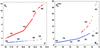 |
Fig. 11 (Left) Angular radius θs and type of the
SMC stars as a function of their apparent magnitude J (in units of
the angular radius of the Sun at 10 kpc). (Right) Maximum angular
radius |
7. Limits on turbulent Galactic hidden gas toward the SMC
Here, the distance of the stars are all the same
z0 + z1 ~ z1 = 62 kpc
(Szewczyk et al. 2009). Therefore the angular
stellar radii θs can be (roughly) estimated from the observed
J magnitude. We used the EROS data (Tisserand et al. 2007; Hamadache et al.
2006; Rahal et al. 2009) to distinguish
between main sequence and red giant branch stars from the REROS
versus (BEROS − REROS)
color-magnitude diagram; then the stellar type is obtained from the absolute magnitude
MJ = J − 5·log (62 000 pc/10 pc)
and θs is derived from Eq. (9) (see Fig. 11, left). With these
ingredients, we can estimate from Eq. (8)
the lowest value of
Rdiff compatible with the measured modulation index
m for each stellar light-curve. Figure 12a shows the cumulative distribution of this variable
, that is
N ∗ (Rd), the number of stars
whose line of sight do not cross a gaseous structure with
Rdiff < Rd. The bimodal
shape of this distribution is caused by the prominence of the red giants in the monitored
population: scintillation is expected to be less contrasted for red giant stars because of
their large radius; therefore, structures with Rdiff ≳ 250 km
cannot induce detectable modulation in the red giant light-curves, and the
values are lower
than 250 km.
The distribution vanishes beyond Rd ~ 800 km because
our limited resolution on the main sequence stars (a few %) prevents us from detecting any
scintillation of gaseous structures with Rdiff > 800 km.
The possible Rdiff domain for the hidden gas clumpuscules
expected from the model of (Pfenniger et al. 1994;
Pfenniger & Combes 1994) and their maximum
contribution to the optical depth are indicated by the gray zone; the minimum
Rdiff (~17 km at
λ = 1.25 μm) for these objects is estimated from
Eq. (1) assuming the clumpuscule’s outer
scale is 30 AU and considering the maximum possible value of the density fluctuation,
mathematically limited by the maximum density (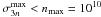 cm-3) (Pfenniger et al. 1994; Pfenniger & Combes 1994).
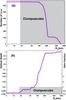 |
Fig. 12 a) N ∗ (Rd), the number of SMC stars (or lines of sight) with no turbulent structure of Rdiff(1.25 μm) < Rd along the line of sight. The gray band shows the allowed Rdiff(1.25 μm) region for clumpuscules (see text). b) The 95% CL maximum optical depth of structures with Rdiff < Rd toward the SMC. The right scale gives the maximum contribution of structures with Rdiff(1.25 μm) < Rd to the Galactic halo (in fraction); the gray zone gives the possible region for the hidden gas clumpuscules. |
From the distribution of N ∗ (Rd),
one can infer limits on the scintillation optical depth
τ1.25 μm(Rd)
as it is defined in Sect. 2.5. Indeed
N ∗ (Rd) is the number of lines of
sights (l.o.s.) that do not cross structures with
Rdiff < Rd. Defining
Nbehind as the total number of monitored l.o.s. through the
nebula (all monitored stars in the present case because we are searching for invisible gas),
the upper limit on the optical depth
τ1.25 μm(Rd) is
the upper limit on the ratio  .
The 95% statistical upper limit on p is given by the classical confidence
interval i.e.2:
.
The 95% statistical upper limit on p is given by the classical confidence
interval i.e.2:
-
if N ∗ (Rd) and Nbehind − N ∗ (Rd) are both larger than 4, then
 (10)
(10) -
if N ∗ (Rd) ≤ 4, then
 (11)where
N95%(Rd) is the 95% CL
Poissonian lower limit on
N ∗ (Rd);
(11)where
N95%(Rd) is the 95% CL
Poissonian lower limit on
N ∗ (Rd); -
if Nbehind − N ∗ (Rd) ≤ 4, then
![\begin{equation} \tau_{\lambda}(R_{\rm d}) < \frac{[N_{\rm behind}-N_*(R_{\rm d})]_{95\%}}{N_{\rm behind}}, \end{equation}](/articles/aa/full_html/2011/01/aa15260-10/aa15260-10-eq229.png) (12)where
[ Nbehind − N ∗ (Rd) ] 95%
is the 95% CL Poissonian upper limit on
Nbehind − N ∗ (Rd).
(12)where
[ Nbehind − N ∗ (Rd) ] 95%
is the 95% CL Poissonian upper limit on
Nbehind − N ∗ (Rd).
The expected optical depth is proportional to the total mass of gas. In Pfenniger et al. (1994) the clumpuscules are expected to cover less than ~1% of the sky; this means that the maximum optical depth should be ~0.01 assuming a Galactic halo completely made of gaseous clumpuscules. Therefore, we can interpret our optical depth limit as the upper limit of the contribution of turbulent gaseous structures with Rdiff(1.25 μm) < Rd, expressed in fraction of the halo (right scale in Fig. 12b).
Our upper limit does not yet seriously constrain the model with clumpuscules, but we can extrapolate these results to define a strategy to reach a significant sensitivity. Our monitored stellar population is dominated by red giant stars that would give a lower scintillation signal than smaller stars from the main sequence. This could only be compensated by achieving an excellent photometric precision on the red giants. An easier way to improve a hypothetic signal would be to use V passband instead of J. In our test, the use of J filter was imposed by the choice of the SOFI detector, the only one available with a fast readout. According to the ESO exposure time calculator (ESO-SOFI 2007), the same precision we obtained in J for the red giants can be reached for A0 stars in V with the same exposure time (10 s). Therefore, we can extrapolate that an exposure of ~106 star × hour (about 100 times more than our test) obtained with the same type of telescope (NTT) using the V passband (around the maximum of stellar emission) should provide enough sensitivity to significantly constrain the turbulent gas component of the Galactic halo.
8. Limits on the gas structuration in the nebulae
For our study of known nebulae, the distance z0 to the gas is
known, but not the star-by-star z1 distances. We first make the
hypothesis that the stellar population behind the clouds (whose light is absorbed and
diffracted) is the same as the population which is not – or much less – obscured (the
so-called control population, see Fig. 7). Toward B68
the red giant stars are distinguished from the main sequence stars with our own
J image, also taken with the NTT-SOFI detector, through the
Ks versus
(J − Ks) diagram. Using Eq. (9), we established the
Ks to relation,
providing the maximum angular radius of a main sequence or red giant star located beyond
4 kpc with Ks apparent magnitude (Fig. 11 right). We conservatively use this angular radius in Eq. (8) to estimate
. The study of the
population behind the dust is complicated by the fact that the stars are obscured. In the
case of B68 we were able to correct the apparent magnitudes for the absorption in
Ks band; we used the
AV absorption map from (Alves et al. 2001) and the relation
AK/AV = 0.089
(Ojha et al. 2000; Glass et al. 1999) to extract AK and
deduce the dereddened magnitudes Ks. Using the relation of
Fig. 11 (right) with these corrected magnitudes, we
extract for each star
behind the dust.
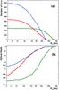 |
Fig. 13 a) N ∗ (Rd), the number of directions with no turbulent structure of Rdiff(2.16 μm) < Rd along the line of sight toward the obscured regions of B68 (green), cb131 (blue) and toward the Circinus nebula (red). b) The 95% CL maximum optical depth of structures with Rdiff(2.16 μm) < Rd. |
Because there is no absorption map for bc131 and the Circinus nebula, we conservatively
used the highest possible value of  (corresponding to a B3 type star at 4.5 kpc).
Figure 13 shows the cumulative
distributions and
the upper limits on
τ2.16 μm(Rd)
for the obscured regions of B68 and bc131 (the search regions from Fig. 7) and over the complete field of the Circinus nebula, which has
indistinct boundaries. The best limits are naturally obtained toward B68, as a consequence
of the better knowledge of the stellar sizes. The shape of the cumulative
distributions
differs from the one obtained toward the SMC, because the contribution of (big) red giant
stars is smaller.
We can now interpret our limits on Rdiff to constrain the global structure of the nebulae, and specifically put limits on the existence and the structure of local turbulent dense cores (cells) within the nebulae (see Lada et al. 2007; and Racca 2009).
-
Probing the global structure? If the nebula is a simple object described by a single Kolmogorov turbulence law, characterized by an outer scale of Lz ~ 17 000 AU (maximum depth of gas crossed by the light in B68), then the minimum expected value of Rdiff is deduced from Eq. (1), where σ3n is limited by nmax the maximum molecular density. This maximum is estimated to be 2.61 × 105 cm-3 for B68 (Hotzel et al. 2002). Using this constraint and the maximum outer scale value in (1) gives for B68
![\begin{eqnarray} &&\!\!\! R_{\rm diff}(2.16~\mu{\rm m})> \nonumber \\ &&\!\!\! 263\, km \left[\frac{2.16~\mu{\rm m}}{1~\mu{\rm m}}\right]^{\frac{6}{5}} \left[\frac{17\,000\,{\rm AU}}{10\,{\rm AU}}\right]^{-\frac{1}{5}}\! \left[\frac{2.61\!\times\! 10^{5}\,{\rm cm}^{-3}}{10^{9}\,{\rm cm}^{-3}}\right]^{-\frac{6}{5}} \nonumber \\ &&\hspace*{19mm} >3.\times 10^6~{\rm km}. \end{eqnarray}](/articles/aa/full_html/2011/01/aa15260-10/aa15260-10-eq251.png) (13)For
cb131, the same calculation based on data from (Bacmann
et al. 2000) gives
Rdiff(2.16 μm) > 4.2 × 10⁶ km.
These large diffusion radii, which are owing to the weakness of the power spectrum at
small scales, are much too large to induce any observable scintillation effect on any
type of stars. Indeed, because
θs > θ(R⊙ at 10 kpc),
Eq. (3) gives
Rs/Rref > 3100 at
λ = 2.16 μm, and the expected modulation index
is completely negligible (out of scale in Fig. 3).
(13)For
cb131, the same calculation based on data from (Bacmann
et al. 2000) gives
Rdiff(2.16 μm) > 4.2 × 10⁶ km.
These large diffusion radii, which are owing to the weakness of the power spectrum at
small scales, are much too large to induce any observable scintillation effect on any
type of stars. Indeed, because
θs > θ(R⊙ at 10 kpc),
Eq. (3) gives
Rs/Rref > 3100 at
λ = 2.16 μm, and the expected modulation index
is completely negligible (out of scale in Fig. 3). -
Probing local sub-structures? In contrast, local turbulent dense cores with much smaller diffusion radii could potentially produce observable scintillation. Therefore our upper limits on scintillation can be interpreted as upper limits on the existence of turbulent cells with Rdiff(2.16 μm) < 350 km within the volume of the nebula. Using Eq. (1), it can be interpreted as limits on the distribution of the product
![\begin{equation} \left[\frac{\sigma_{3n}}{\rm 10^{9}\, cm^{-3}}\right] \left[\frac{L_z}{\rm 10\ AU}\right]^{\frac{1}{6}} = \left[\frac{R_{\rm diff}(2.16~\mu{\rm m})}{\rm 663\, km}\right]^{-\frac{5}{6}} \end{equation}](/articles/aa/full_html/2011/01/aa15260-10/aa15260-10-eq256.png) (14)along
the lines of sight; thanks to the small exponent of
Lz, a rough hypothesis for the core
size would allow one to extract upper limits on the frequency of cores with a density
dispersion higher than a given value σ3n.
No conclusion can be infered for structures with
Rdiff > 350 km, because they cannot produce a
detectable scintillation in our sample because of our limited photometric precision on
the small stars.
(14)along
the lines of sight; thanks to the small exponent of
Lz, a rough hypothesis for the core
size would allow one to extract upper limits on the frequency of cores with a density
dispersion higher than a given value σ3n.
No conclusion can be infered for structures with
Rdiff > 350 km, because they cannot produce a
detectable scintillation in our sample because of our limited photometric precision on
the small stars.
9. Conclusions and perspectives
The aim of the test was to study the feasibility of a systematic search for scintillation. We were lucky enough to find a stochastic variable light-curve that is compatible with a scintillation effect; but considering the low probability of such an event, which is related to the low density of the nebulae, a program of synchroneous multicolor and multi-epoch observations is necessary to obtain a convincing signature of the effect.
From our search for invisible gas toward the SMC, we conclude that an ambitious program using a wide field, fast readout camera at the focal plane of a >4 m telescope should either discover turbulent gas in the halo, or exclude this type of hidden baryonic matter. With such a setup, significant results should be obtained with an exposure of ~106 star × hour in V passband.
The hardware and software techniques required for scintillation searches are available just now, and a reasonably priced dedicated project could be operational within a few years. Alternatives under study are the use of the data from the LSST project and from the GAIA mission. If a scintillation indication is found in the future, one will have to consider a much more ambitious project involving synchronized telescopes, a few thousand kilometers apart. Such a project would allow one to temporally and spatially sample an interference pattern, unambiguously providing the refractive length scale Rref, the speed, and the dynamics of the scattering medium.
The first formula gives the upper limit of the 90% CL interval for the p value (see classical texbooks like Ventsel 1973); therefore the probability that the true p value is higher than the upper limit of this interval is 5%.
Acknowledgments
We are grateful to the IPM for supporting F. Habibi during his stay in Tehran. We thank Prof. P. Schwemling for his help in the determination of the variable star parameters, J.-F. Glicenstein, F. Cavalier and P. Hello for their participation to discussions. We thank Prof. J.-F. Alves for providing us with the B68 absorption map. We are grateful to the referee for his constructive remarks that allowed us to significantly improve this article.
References
- Alcock, C., Allsman, R. A., Alves, D., et al. 2000, ApJ, 542, 281 [NASA ADS] [CrossRef] [Google Scholar]
- Alves, J., Lada, C. J., & Lada, E. A. 2001, Nature, 409, 159 [NASA ADS] [CrossRef] [PubMed] [Google Scholar]
- Ansari, R. 1996, Vistas in Astronomy, 40, No. 4 [Google Scholar]
- Bacmann, A., André, P., Puget, J.-L., et al. 2000, A&A, 361, 555 [NASA ADS] [Google Scholar]
- Caldwell, J., & Coulson, I. 1986, MNRAS, 218, 223 [NASA ADS] [CrossRef] [Google Scholar]
- Cox, A. N. 2000, Allen’s Astrophysical Quantities, 4th ed. (Springer) [Google Scholar]
- De Paolis, F., Ingrosso, G., Jetzer, Ph., & Roncadelli, M. 1995, Phys. Rev. Lett., 74, 14 [NASA ADS] [CrossRef] [PubMed] [Google Scholar]
- De Paolis, F., Ingrosso, G., Jetzer, Ph., & Roncadelli, M. 1998, ApJ, 500, 59 [NASA ADS] [CrossRef] [Google Scholar]
- Dravins, D., Lindegren, L., Mezey, E., & Young, A. T. 1997, Pub. Ast. Soc. Pacific, 109 (parts I and II) (part III), 1998, 110 [Google Scholar]
- ESO-GASGANO User’s Manual, Amico, P., Kornweibel, N., & Zamparelli, M. 2001, Doc. No. VLT-PRO-ESO-19000-1932 [Google Scholar]
- ESO SOFI Exposure Time Calculator, Version 3.2.1. 2007, http://www.eso.org/observing/etc/ [Google Scholar]
- Georgelin, Y. M., Amram, P., Georgelin, Y. P., et al. 1994, A&AS, 108, 513 [NASA ADS] [Google Scholar]
- Glass, I. S., Ganesh, S., Alard, C., et al. 1999, MNRAS, 308, 127 [NASA ADS] [CrossRef] [Google Scholar]
- Hamadache, C., Le Guillou, L., Tisserand, P., et al. 2006, A&A, 454, 185 [NASA ADS] [CrossRef] [EDP Sciences] [Google Scholar]
- Hotzel, S., Harju, J., Juvela, M., et al. 2002, A&A, 391, 275 [NASA ADS] [CrossRef] [EDP Sciences] [Google Scholar]
- Johnson, H. L. 1966, ARA&A, 4, 193 [NASA ADS] [CrossRef] [Google Scholar]
- Lada, C. J., Alves, J. F., & Lombardi, M. 2007, Near-Infrared Extinction and Molecular Cloud Structure, Protostars and Planets V, 3 [Google Scholar]
- Lovelace, R. V. E. 1970, Ph.D. Thesis, Cornell University [Google Scholar]
- Lovelace, R. V. E., Salpeter, E. E., Sharp, L. E., & Harris, D. E. 1970, ApJ, 159, 1047 [NASA ADS] [CrossRef] [Google Scholar]
- Lyne, A. G., & Graham-Smith., F. 1998, Pulsar Astronomy (Cambridge University Press) [Google Scholar]
- Moniez, M. 2003, A&A, 412, 105 [NASA ADS] [CrossRef] [EDP Sciences] [Google Scholar]
- Moniez, M. 2010, Gen. Rel. Grav., 42, 2047 [NASA ADS] [CrossRef] [Google Scholar]
- Narayan, R. 1992, Phil. Trans. R. Soc. Lond. A, 341, 151 [Google Scholar]
- Ojha, D. K., Omont, A., Ganesh, S., et al. 2000, J. Astrophys. Astr., 21, 77 [NASA ADS] [CrossRef] [Google Scholar]
- Pfenniger, D., & Combes, F. 1994, A&A, 285, 94 [NASA ADS] [Google Scholar]
- Pfenniger, D., Combes, F., & Martinet, L. 1994, A&A, 285, 79 [NASA ADS] [Google Scholar]
- Racca, G. A., Vilas-Boas, J. W. S., & De la Reza, R. 2009, ApJ, 703, 1444 [NASA ADS] [CrossRef] [Google Scholar]
- Rahal, Y. R., Afonso, C., Albert, J.-N., et al. 2009, A&A, 500, 1027 [NASA ADS] [CrossRef] [EDP Sciences] [Google Scholar]
- Russeil, D., Amram, P., Georgelin, Y. P., et al. 1998, A&AS, 130, 119 [NASA ADS] [CrossRef] [EDP Sciences] [Google Scholar]
- Skrutskie, M. F., Cutri, R. M., Stiening, R., et al. 2006, AJ, 131, 1163 [NASA ADS] [CrossRef] [Google Scholar]
- Sterken, C., & Jaschek, C. 1996, Light Curves of Variable Stars, a pictorial Atlas (Cambridge University Press) [Google Scholar]
- Szewczyk, O., Pietrzynski, G., Gieren, W., et al. 2009, AJ, 138, 1661 [NASA ADS] [CrossRef] [Google Scholar]
- Tisserand, P. 2004, Ph.D. Thesis, Université de Nice-Sophya Antipolis CEA DAPNIA-04-09-T [Google Scholar]
- Tisserand, P., Le Guillou, L., Afonso, C., et al. 2007, A&A, 469, 387 [NASA ADS] [CrossRef] [EDP Sciences] [Google Scholar]
- Ventsel, H. 1973, Théorie des probabilités (Moscou: Mir) [Google Scholar]
- Wyrzykowski, L., Kozlowski, S., Skowron, J., et al. 2010, MNRAS, 407, 189 [NASA ADS] [CrossRef] [Google Scholar]
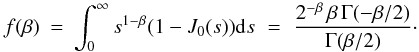
Appendix A: Connection between the diffusion radius and the gas structuration
We consider a gaseous medium characterized by a cell with size
(Lx,Ly,Lz).
An electromagnetic plane wave propagating along z and crossing the medium
is distorted. The distorsion is caused by the variation of the column density along the
propagation of the light and can be described by a two-dimensional phase delay
φ(x,y). We use the phase structure function to
characterize the variations of the phase as follows: ![\appendix \setcounter{section}{1} \begin{eqnarray} \label{dphi} D_{\phi}(x,y) & = & \left\langle\left(\phi\left(x'+x,y'+y\right)-\phi\left(x',y'\right)\right)^2\right\rangle \\ & = & 2 \left[\left\langle\phi^2\left(x',y'\right)\right\rangle - \left\langle\phi(x'+x,y'+y) \phi(x',y')\right\rangle\right] \nonumber \\ & = & 2 \left[\xi_{\phi}(0,0) - \xi_{\phi}(x,y)\right], \nonumber \end{eqnarray}](/articles/aa/full_html/2011/01/aa15260-10/aa15260-10-eq262.png) (A.1)where
ξφ(x,y) is the correlation
function of the screen phase and is related to the phase spectral density
Sφ(qx,qy)
(power spectrum per volume unit) through the Fourier transform as
(A.1)where
ξφ(x,y) is the correlation
function of the screen phase and is related to the phase spectral density
Sφ(qx,qy)
(power spectrum per volume unit) through the Fourier transform as 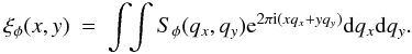 (A.2)Substituting
Eq. (A.2) in (A.1) we obtain
(A.2)Substituting
Eq. (A.2) in (A.1) we obtain  (A.3)The
relation between the two-dimensional spectrum of the phase,
Sφ(qx,qy)
and the three-dimensional spectrum of the number density fluctuations has been derived for
a plasma by Lovelace (Lovelace 1970; Lovelace et al. 1970). Here we extend the concept to
the optical wavelength for a medium of molecular gas:
(A.3)The
relation between the two-dimensional spectrum of the phase,
Sφ(qx,qy)
and the three-dimensional spectrum of the number density fluctuations has been derived for
a plasma by Lovelace (Lovelace 1970; Lovelace et al. 1970). Here we extend the concept to
the optical wavelength for a medium of molecular gas:  (A.4)where
S3δn(qx,qy,qz)
is the spectrum of the density fluctuations of the molecular gas in three dimensions
(δn = n − ⟨ n ⟩ ),
α is the average polarizability of the molecules and
Lz is the thickness of the medium along
the line of sight.
(A.4)where
S3δn(qx,qy,qz)
is the spectrum of the density fluctuations of the molecular gas in three dimensions
(δn = n − ⟨ n ⟩ ),
α is the average polarizability of the molecules and
Lz is the thickness of the medium along
the line of sight.
Assuming the gaseous medium to be isotropically turbulent, the 3D spectral density obeys
a power law relation within the turbulence inertial range:  (A.5)where
 ,
β = 11/3 is taken for the Kolmogorov turbulence,
,
β = 11/3 is taken for the Kolmogorov turbulence,
 is the
turbulence strength parameter and Lout and
Lin are the outer and inner scales of the turbulence
respectively. By substituting Eqs. (A.5)
and (A.4) in Eq. (A.3), we compute the phase structure function
in the polar coordinate system:
is the
turbulence strength parameter and Lout and
Lin are the outer and inner scales of the turbulence
respectively. By substituting Eqs. (A.5)
and (A.4) in Eq. (A.3), we compute the phase structure function
in the polar coordinate system: 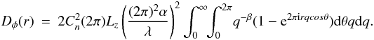 The
integration results in
The
integration results in 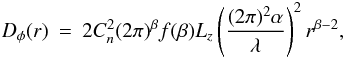 (A.6)where
 For
the Kolmogorov turbulence
f(β = 11/3) ~ 1.118.
For
the Kolmogorov turbulence
f(β = 11/3) ~ 1.118.
We define the diffusion radius Rdiff as the transverse scale
for which
Dφ(Rdiff) = 1 rad.
Rdiff is directly obtained from Eq. (A.6): ![\appendix \setcounter{section}{1} \begin{eqnarray} R_{\rm diff} &=& [2 C_n^2 (2\pi)^{\beta+4} f(\beta) L_z \alpha^2 \lambda^{-2}]^{1/(2-\beta)}. \label{rdiff} \end{eqnarray}](/articles/aa/full_html/2011/01/aa15260-10/aa15260-10-eq284.png) (A.7)We
will now link the turbulence parameter to the
dispersion of the density fluctuation. From Parseval’s theorem the dispersion of the
density fluctuation is equal to the auto-correlation function at origin:
(A.7)We
will now link the turbulence parameter to the
dispersion of the density fluctuation. From Parseval’s theorem the dispersion of the
density fluctuation is equal to the auto-correlation function at origin:
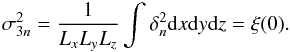 (A.8)On the other hand the
auto-correlation is equal to the integration over the spectrum in the Fourier space
(A.8)On the other hand the
auto-correlation is equal to the integration over the spectrum in the Fourier space
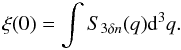 (A.9)Using Eq. (A.5), the dispersion of the density
fluctuations is related to as
(A.9)Using Eq. (A.5), the dispersion of the density
fluctuations is related to as
 (A.10)Assuming
Lz = Lout ≫ Lin,
for β = 11/3, we estimate as
(A.10)Assuming
Lz = Lout ≫ Lin,
for β = 11/3, we estimate as
 (A.11)Finally
by substituting Eq. (A.11) in (A.7), Rdiff is
obtained in terms of the cloud’s parameters and the wavelength as
(A.11)Finally
by substituting Eq. (A.11) in (A.7), Rdiff is
obtained in terms of the cloud’s parameters and the wavelength as
![\appendix \setcounter{section}{1} \begin{eqnarray} R_{\rm diff}\!=\! 231.1\,{\rm km} \left[\frac{\alpha}{\alpha_{\rm H_2}}\right]^{-\frac{6}{5}} \! \left[\!\frac{\lambda}{1\,\mu{\rm m}}\right]^{\frac{6}{5}} \! \left[\!\frac{L_z}{\rm 10\, AU}\right]^{-\frac{1}{5}} \! \left[\frac{\sigma_{3n}}{\rm 10^9\, cm^{-3}}\right]^{-\frac{6}{5}}\!\!\!\!\!\! , \end{eqnarray}](/articles/aa/full_html/2011/01/aa15260-10/aa15260-10-eq290.png) (A.12)where
αH2 = 0.802 × 10⁻²⁴ cm3 is
the polarisability of molecule H2.
(A.12)where
αH2 = 0.802 × 10⁻²⁴ cm3 is
the polarisability of molecule H2.
Appendix B: Limitations of the photometric precision
In our photometric optimization, we found that the photometric precision on unblended
stars was limited by several factors. First, the PSF of very bright stars significantly
differs from the ideal Gaussian and the photometric precision on these stars is seriously
affected. Second, the best photometric precision does not follow the naive expectation
assuming only Poissonian noise. For stars fainter than
Ks = 14.6 (or J = 16.6) we were able to
reproduce the behavior of the PSF fit χ2 and of the fitted
flux uncertainties by assuming that the relative uncertainty
σi,j on a pixel content results from the
combination of the Poissonian fluctuations of the number of photoelectrons
 ,
and of a systematic uncertainty (i.e. not changing with time, but depending on the pixel)
due to the flat-fielding procedure:
,
and of a systematic uncertainty (i.e. not changing with time, but depending on the pixel)
due to the flat-fielding procedure:
![\appendix \setcounter{section}{2} \begin{equation} \sigma_{i,j}^2=\frac{1}{N_{i,j}^{\gamma {\rm e}}}+\left[\frac{\Delta C_{i,j}}{C_{i,j}}\right]^2, \end{equation}](/articles/aa/full_html/2011/01/aa15260-10/aa15260-10-eq299.png) (B.1)where
is the total number of photoelectrons (from the fitted star and the –
usually dominant – sky background), and
(B.1)where
is the total number of photoelectrons (from the fitted star and the –
usually dominant – sky background), and  is the uncertainty of the flat-field coefficient for pixel (i,j). From
the comparison of two flat-fields taken at different epochs, we estimated that
is the uncertainty of the flat-field coefficient for pixel (i,j). From
the comparison of two flat-fields taken at different epochs, we estimated that
 (both
in KS and in J). A third source of noise in
J comes from a residual fringing; we measured that fringes contribute
to a ~40% increase of the Poissonian fluctuation
(both
in KS and in J). A third source of noise in
J comes from a residual fringing; we measured that fringes contribute
to a ~40% increase of the Poissonian fluctuation
 in a domain size comparable to the PSF width because of their small spatial scale.
We conclude that the contribution of the Poissonian noise dominates the error when the flux from the star plus the total sky background within the PSF fitting domain is small (~2000 ADU = 10 600γe). For brighter stars or for stars located in a dusty environment (producing a large sky IR background), the second – systematic – term dominates.
All Tables
All Figures
|
Fig. 1 Left: a 2D stochastic phase screen (gray scale) from a simulation of gas affected by Kolmogorov-type turbulence. Right: the illumination pattern from a point source (left) after crossing such a phase screen. The distorted wavefront produces structures at scales of ~Rdiff(λ) and Rref(λ) on the observer’s plane. |
| In the text | |
|
Fig. 2 Simulated illumination map at λ = 2.16 μm on Earth from a point source (up-left)- and from a K0V star (rs = 0.85 R⊙, MV = 5.9) at z1 = 8 kpc (right). The refracting cloud is assumed to be at z0 = 160 pc with a turbulence parameter Rdiff(2.16 μm) = 150 km. The circle shows the projection of the stellar disk (with radius RS = rs × z0/z1). The bottom maps are illuminations in the Ks wide band (λcentral = 2.162 μm, Δλ = 0.275 μm). |
| In the text | |
|
Fig. 3 Expected intensity modulation index |
| In the text | |
|
Fig. 4 The four monitored fields, showing the structures of the nebulae and the background stellar densities. From left to right: B68, Circinus, cb131, and the SMC. Up: images from the ESO-DSS2 in R. Down: our corresponding template images (in Ks for B68, cb131 and Circinus, in J for SMC). North is up and East is left. The circles on the B68 images show the position of our selected candidate. |
| In the text | |
|
Fig. 5 Dispersion of the photometric measurements along the light-curves as a function of the mean Ks magnitude (up) and J magnitude (down). Each dot corresponds to one light-curve. In the upper panel, the small black dots correspond to control stars that are not behind the gas; the big blue dots correspond to stars located behind the gas; the big star marker indicates our selected candidate. |
| In the text | |
|
Fig. 6 Seeing distributions of the images towards the four targets. The images with larger seeing than the position of the arrow are discarded. |
| In the text | |
|
Fig. 7 Definition of the control regions (yellow dots) and the search regions (blue dots) toward B68 (left) and cb131 (right). |
| In the text | |
|
Fig. 8 The R = σφ/σint versus Ks (or J) distributions of the light-curves of the monitored stars. The red dots correspond to the most variable light-curves. The green stars indicate two known variable objects toward SMC and our selected candidate toward B68. |
| In the text | |
|
Fig. 9 EROS folded light-curves of cepheids HV1562 (upper-left) and of the EROS object () (right) in BEROS and REROS passbands, with our NTT observations in J (black dots). The lower-left panels show details around our observations. |
| In the text | |
|
Fig. 10 Light-curves for the two nights of observation (top) and images of the selected candidate toward B68 during a low-luminosity phase (middle) and a high-luminosity phase (bottom); North is up, East is left. |
| In the text | |
|
Fig. 11 (Left) Angular radius θs and type of the
SMC stars as a function of their apparent magnitude J (in units of
the angular radius of the Sun at 10 kpc). (Right) Maximum angular
radius |
| In the text | |
|
Fig. 12 a) N ∗ (Rd), the number of SMC stars (or lines of sight) with no turbulent structure of Rdiff(1.25 μm) < Rd along the line of sight. The gray band shows the allowed Rdiff(1.25 μm) region for clumpuscules (see text). b) The 95% CL maximum optical depth of structures with Rdiff < Rd toward the SMC. The right scale gives the maximum contribution of structures with Rdiff(1.25 μm) < Rd to the Galactic halo (in fraction); the gray zone gives the possible region for the hidden gas clumpuscules. |
| In the text | |
|
Fig. 13 a) N ∗ (Rd), the number of directions with no turbulent structure of Rdiff(2.16 μm) < Rd along the line of sight toward the obscured regions of B68 (green), cb131 (blue) and toward the Circinus nebula (red). b) The 95% CL maximum optical depth of structures with Rdiff(2.16 μm) < Rd. |
| In the text | |
Current usage metrics show cumulative count of Article Views (full-text article views including HTML views, PDF and ePub downloads, according to the available data) and Abstracts Views on Vision4Press platform.
Data correspond to usage on the plateform after 2015. The current usage metrics is available 48-96 hours after online publication and is updated daily on week days.
Initial download of the metrics may take a while.