| Issue |
A&A
Volume 520, September-October 2010
|
|
|---|---|---|
| Article Number | A26 | |
| Number of page(s) | 14 | |
| Section | Interstellar and circumstellar matter | |
| DOI | https://doi.org/10.1051/0004-6361/200913454 | |
| Published online | 23 September 2010 | |
Interstellar absorptions towards the LMC:
small-scale density variations in Milky Way disc gas
S. Nasoudi-Shoar1 - P. Richter2 - K. S. de Boer1 - B. P. Wakker3
1 - Argelander-Institut für Astronomie,
Universität Bonn, Auf dem Hügel 71, 53121 Bonn, Germany
2 - Institut für Physik und Astronomie, Universität Potsdam,
Haus 28, Karl-Liebknecht-Str. 24/25, 14476 Golm, Germany
3 - Department of Astronomy, University of Wisconsin, 475 N Charter St,
Madison, WI 53706, USA
Received 12 October 2009 / Accepted 1 June 2010
Abstract
Observations show that the interstellar medium (ISM) contains
sub-structure on scales less than 1 pc, detected in the form
of spatial and temporal variations in column densities or optical
depth. Despite the number of detections, the nature and ubiquity of the
small-scale structure in the ISM is not yet fully understood. We use UV
absorption data mainly from the Far Ultraviolet Spectroscopic Explorer
(FUSE) and partly from the Space Telescope Imaging Spectrograph (STIS)
of six Large Magellanic Cloud (LMC) stars (Sk -67![]() 111,
LH 54-425, Sk -67
111,
LH 54-425, Sk -67![]() 107, Sk -67
107, Sk -67![]() 106,
Sk -67
106,
Sk -67![]() 104,
and Sk -67
104,
and Sk -67![]() 101)
that are all located within 5
101)
that are all located within 5![]() of each other, and analyse the physical properties of the Galactic disc
gas in front of the LMC on sub-pc scales. We analyse absorption lines
of a number of ions within the UV spectral range. Most importantly,
interstellar molecular hydrogen, neutral oxygen, and fine-structure
levels of neutral carbon have been used in order to study changes in
the density and the physical properties of the Galactic disc gas over
small angular scales. At an assumed distance of 1 kpc, the 5
of each other, and analyse the physical properties of the Galactic disc
gas in front of the LMC on sub-pc scales. We analyse absorption lines
of a number of ions within the UV spectral range. Most importantly,
interstellar molecular hydrogen, neutral oxygen, and fine-structure
levels of neutral carbon have been used in order to study changes in
the density and the physical properties of the Galactic disc gas over
small angular scales. At an assumed distance of 1 kpc, the 5![]() separation between Sk -67
separation between Sk -67![]() 111 and Sk -67
111 and Sk -67![]() 101 implies a
linear extent of 1.5 pc.
101 implies a
linear extent of 1.5 pc.
We report on column densities of H2, C I,
N I, O I,
Al II, Si II,
P II, S III,
Ar I, and Fe II
in our six lines of sight, as well as C I*,
C I**, Mg II,
Si IV, S II,
Mn II, and Ni II
for four of them. While most species do not show any significant
variation in their column densities, we find an enhancement of almost
2 dex for H2 from Sk -67![]() 111 to
Sk -67
111 to
Sk -67![]() 101,
accompanied by only a small variation in the O I column
density. Based on the formation-dissociation equilibrium, we trace
these variations to the actual density variations in the molecular gas.
On the smallest spatial scale of <0.08 pc, between
Sk -67
101,
accompanied by only a small variation in the O I column
density. Based on the formation-dissociation equilibrium, we trace
these variations to the actual density variations in the molecular gas.
On the smallest spatial scale of <0.08 pc, between
Sk -67![]() 107
and LH 54-425, we find a gas density variation of a factor
of 1.8. The line of sight towards LH 54-425 does not
follow the relatively smooth change seen from Sk -67
107
and LH 54-425, we find a gas density variation of a factor
of 1.8. The line of sight towards LH 54-425 does not
follow the relatively smooth change seen from Sk -67![]() 101 to
Sk -67
101 to
Sk -67![]() 111,
suggesting that sub-structure might exist on a smaller spatial scale
than the linear extent of our sight-lines.
111,
suggesting that sub-structure might exist on a smaller spatial scale
than the linear extent of our sight-lines.
The results show that we sample a mix of both neutral and
ionised gas in our six lines of sight. Towards Sk -67![]() 101 to
Sk -67
101 to
Sk -67![]() 107,
we derive the temperature
107,
we derive the temperature ![]() K
for the inner self-shielded part of the gas based on the rotational
excitation levels of H2, and an average density
of
K
for the inner self-shielded part of the gas based on the rotational
excitation levels of H2, and an average density
of ![]() ,
typical of that for CNM. The gas towards LH 54-425 and
Sk -67
,
typical of that for CNM. The gas towards LH 54-425 and
Sk -67![]() 111
shows different properties, and
111
shows different properties, and ![]() K.
Our observations suggest that the detected H2 in
these six lines of sight (with the extent of <1.5 pc)
is not necessarily physically connected, but that we are sampling
molecular cloudlets with pathlengths <0.1-1.8 pc and
possibly different densities.
K.
Our observations suggest that the detected H2 in
these six lines of sight (with the extent of <1.5 pc)
is not necessarily physically connected, but that we are sampling
molecular cloudlets with pathlengths <0.1-1.8 pc and
possibly different densities.
Key words: ISM: structure - ISM: molecules - ultraviolet: ISM - techniques: spectroscopic - Galaxy: disc
1 Introduction
Recent studies of the interstellar medium have shown a number of observed variations on scales smaller than 1 pc, indicating the existence of small-scale structure. These have been reported in the form of temporal variations and differences in column densities over small spatial scales.
Interferometric data of neutral hydrogen in 1976 showed variations in H I over small scales (Dieter et al. 1976). Since then a number of studies of small-scale structures in H I have been performed, by 21-cm absorption lines against pulsars with time variability (e.g., Clifton et al. 1988; Frail et al. 1994), sampling the gas on scales of tens to hundreds of AUs, or using interferometric observations with the Very Long Baseline Array (VLBA) (e.g., Faison & Goss 2001) finding optical depth variations on about the same scales.
Optical spectra at high spectral resolution have been taken of stars in globular clusters, providing a grid of very close sight-lines (angular scales of only few arcsec) to detect structure in interstellar gas on scales down to 0.01 pc. In these studies column density variations have been found in mainly Ca II and Na I lines, and in differential reddening (e.g. Bates et al. 1990; Meyer & Lauroesch 1999; Bates et al. 1995; Andrews et al. 2001; Cohen 1978; Bates et al. 1991).
Using nearby binaries and multiple star systems with separations <20 arcsec, the smallest projected scales have been probed (e.g., Watson & Meyer 1996; Meyer 1990; Lauroesch et al. 2000).
When measurements on small-scale structure were repeated, temporal variations have been found in several cases. Examples have been presented in the above cited investigations by, e.g., Lauroesch et al. (2000), and Lauroesch & Meyer (2003). In some other cases, where a proper motion star was the target, the repeated observations have revealed the spatial variations in the gas on scales smaller than the ones provided by multiple stars and binaries, as the lines of sight sample different parts of the same cloud at different times (Welty & Fitzpatrick 2001; Welty 2007).
Despite the number of detections, the nature of these small-scale structures and their ubiquity is still a subject of study. It has not always been clear whether they reflect the variation in H I column density, or whether they are caused by changes in the physical conditions of the gas over small scales.
However, some explanations have been suggested for the ISM model consisting of fine scale structures, such as filamentary structures (Heiles 1997), fractal geometries driven by turbulence (Elmegreen 1997), or a separate population of cold self-graviting clouds (Draine 1998; Walker & Wardle 1998; Wardle & Walker 1999).
In absorption line spectroscopy most cases of temporal or spatial small-scale structures are observed in optical high-resolution spectra which, however, often provide little information on the physical conditions in the gas. Using UV spectra, valuable information can be gained about the physical properties of the gas. From fine structure levels of C I, Welty (2007) discovered that the observed variations in Na I and Ca II lines towards HD 219188 reflect the variation in the density and ionisation in the gas, and do not refer to high-density clumps. A different approach was used by Richter et al. (2003b,a) who found, using the many absorption lines of molecular hydrogen in the Lyman and Werner bands, that the molecular gas in their studied lines of sight resides in compact filaments, which possibly correspond to the tiny-scale atomic structures in the diffuse ISM (Richter et al. 2003a).
The Large Magellanic Cloud (LMC) has many bright stars with
small angular separation on the sky, and provides a good background for
studying the gas in the disc and the halo of the Milky Way at small
scales. Here we have chosen the six LMC stars Sk -67![]() 111,
LH 54-425, Sk -67
111,
LH 54-425, Sk -67![]() 107, Sk -67
107, Sk -67![]() 106,
Sk -67
106,
Sk -67![]() 104,
and Sk -67
104,
and Sk -67![]() 101,
with small angular separations to study the structure of that
foreground gas. We refer the interested reader to Danforth
et al. (2002) for an atlas of FUSE spectra of the
LMC sight-lines.
101,
with small angular separations to study the structure of that
foreground gas. We refer the interested reader to Danforth
et al. (2002) for an atlas of FUSE spectra of the
LMC sight-lines.
This paper is organised as follows: In Sect. 2 we describe the data used in this work. In Sect. 3 we explain the LMC sight-line and the methods used to gain information from the spectra. In Sect. 4 and Sect. 5 respectively we discuss the results for molecular hydrogen and metal absorption. In Sect. 6 we derive a density relation based on H2 and O I to investigate the density variations within the sight-lines, and combine that with the derived average density from the C I excitation to understand the properties of the gas. We discuss the results and interpretations in Sect. 7.
![\begin{figure}
\par\includegraphics[scale=0.65]{3454f1.ps}
\end{figure}](/articles/aa/full_html/2010/12/aa13454-09/img15.png)
|
Figure 1:
H |
| Open with DEXTER | |
2 Data
We used far ultraviolet (FUV) absorption line data from the Far Ultraviolet Spectroscopic Explorer (FUSE) with relatively high S/N to analyse the spectral structure in six lines of sight with small angular separations. For four of our sight-lines high-resolution Space Telescope Imaging Spectrograph (STIS) observations were also available. In total we cover the wavelength range 905-1730 Å, where we can find most electronic transitions of many atomic species and molecular hydrogen.
Table 1: Information about the FUSE data as retrieved from the MAST archive.
The FUSE instrument consists of four co-aligned telescopes and two micro-channel plate detectors, one coated with Al+LiF, the other with SiC. Each has their maximum efficiency in different parts of the spectral range. The spectral data have a resolution of about 20 km s-1 (FWHM), and cover the wavelength range 905-1187 Å, of which 905-1100 Å are by the SiC coatings and 1000-1187 Å by the Al+LiF coatings. Each detector is divided into two segments, A and B. For detailed information about the instrument and observations see Moos et al. (2000) and Sahnow et al. (2000).
In the order of right ascension our target stars are:
Sk -67![]() 111,
LH 54-425, Sk -67
111,
LH 54-425, Sk -67![]() 107, Sk -67
107, Sk -67![]() 106,
Sk -67
106,
Sk -67![]() 104,
and Sk -67
104,
and Sk -67![]() 101
(see Fig. 1).
These are all bright stars of spectral types O and B,
lying on an almost straight line at constant declination, and spread
over
101
(see Fig. 1).
These are all bright stars of spectral types O and B,
lying on an almost straight line at constant declination, and spread
over
![]() in RA. Because the stars are separated mainly in their RA, we have
considered the projected separations in that coordinate. The smallest
separation is however between LH 54-425 and Sk -67
in RA. Because the stars are separated mainly in their RA, we have
considered the projected separations in that coordinate. The smallest
separation is however between LH 54-425 and Sk -67![]() 107, which
has almost the same RA, which means that we have to take into account
the true separation of
107, which
has almost the same RA, which means that we have to take into account
the true separation of ![]() (essentially in the declination), when comparing these two sight-lines.
(essentially in the declination), when comparing these two sight-lines.
We retrieved the already reduced data from the MASTa
archive and co-added them separately for each of the four co-aligned
telescopes. For the information about the retrieved data as well as the
properties of the stars, see Table 1. The data were
all reduced with the CALFUSE v3.2.1, except
for the LH 54-425 and Sk -67![]() 106, which were reduced with CALFUSE v3.2.2.
The typical S/N of the data varies for different detector channels and
sight-lines (see Table 2
for more information on the S/N of the FUSE and the STIS data). The
data from the SiC channels have in general lower S/N, while the data
quality is significantly higher for all the FUSE detectors for the
Sk -67
106, which were reduced with CALFUSE v3.2.2.
The typical S/N of the data varies for different detector channels and
sight-lines (see Table 2
for more information on the S/N of the FUSE and the STIS data). The
data from the SiC channels have in general lower S/N, while the data
quality is significantly higher for all the FUSE detectors for the
Sk -67![]() 111
and LH 54-425 sight-lines. Due to the different wavelength
zero points in the calibrated data, the spectra of different stars and
different cameras might shift within
111
and LH 54-425 sight-lines. Due to the different wavelength
zero points in the calibrated data, the spectra of different stars and
different cameras might shift within ![]() 20 km s-1.
This shift however is steady for the whole spectral range and does not
affect the line identification.
20 km s-1.
This shift however is steady for the whole spectral range and does not
affect the line identification.
The STIS observations were part of a programme for studying
the N 51 D superbubble (Wakker et al., in
preparation). Only the stars Sk -67![]() 107, Sk -67
107, Sk -67![]() 106,
Sk -67
106,
Sk -67![]() 104,
and Sk -67
104,
and Sk -67![]() 101
were observed in that programme. STIS provides a better resolution of
6.8 km s-1, and covers the
wavelength range longward of the FUSE spectrum from about 1150 to
1730 Å.
101
were observed in that programme. STIS provides a better resolution of
6.8 km s-1, and covers the
wavelength range longward of the FUSE spectrum from about 1150 to
1730 Å.
3 Handling of spectral data
3.1 LMC sight-line
The line of sight towards the LMC is rather complicated, because it contains several gas components. Knowing the absorption lines in the ISM with their transition wavelengths we are able to identify the different elements, and distinguish the different gas components through their radial velocities.
We followed the comprehensive description given by, e.g., Savage & de Boer
(1981). On a line of sight there is gas in the solar
vicinity, normally seen around ![]() km s-1
(all velocities given are heliocentric
velocities). Next is the intermediate velocity gas around
km s-1
(all velocities given are heliocentric
velocities). Next is the intermediate velocity gas around ![]() +60 km s-1
on essentially all LMC lines of sight; this gas likely is a foreground
intermediate velocity cloud (IVC). Most lines of sight also show the
presence of a high-velocity cloud (HVC) at
+60 km s-1
on essentially all LMC lines of sight; this gas likely is a foreground
intermediate velocity cloud (IVC). Most lines of sight also show the
presence of a high-velocity cloud (HVC) at ![]() km s-1.
The properties of the IVC and HVC will be discussed in Nasoudi-Shoar et
al. (in preparation). Finally, the LMC gas itself shows its presence in
the velocity range between +180 and +300 km s-1.
In this paper we analyse the Milky Way disc component at the velocity
km s-1.
The properties of the IVC and HVC will be discussed in Nasoudi-Shoar et
al. (in preparation). Finally, the LMC gas itself shows its presence in
the velocity range between +180 and +300 km s-1.
In this paper we analyse the Milky Way disc component at the velocity ![]() km s-1,
where the various rotational levels of molecular hydrogen have
relatively strong absorption and allow for a detailed study of the
properties of the gas. The absolute wavelength calibration of the STIS
data is much more reliable, therefore we base our radial velocities on
these data. This reveals an additional weak component at
km s-1,
where the various rotational levels of molecular hydrogen have
relatively strong absorption and allow for a detailed study of the
properties of the gas. The absolute wavelength calibration of the STIS
data is much more reliable, therefore we base our radial velocities on
these data. This reveals an additional weak component at ![]() km s-1,
which we describe briefly, while we concentrate on the analysis of the
strong disc component. We refer to the absorptions with similar radial
velocity as parts of the same cloud.
km s-1,
which we describe briefly, while we concentrate on the analysis of the
strong disc component. We refer to the absorptions with similar radial
velocity as parts of the same cloud.
3.2 Column-density measurements
The continua of the spectra consist of the spectral structures from the background stars with broad lines and P-Cygni profiles. Before measuring the equivalent widths we estimated a continuum level by eye, and normalised the spectra to unity with the programme SPECTRALYZOR (Marggraf 2004). In this way we eliminated the large scale variation of the continuum as well as the possible variations on scales less than 1 Å. The absorption lines from those parts of the spectra where the continuum placement is highly uncertain were considered with special caution or were excluded from the final analysis.
For each velocity component the equivalent width of the absorption was measured either by integrating the pixel to pixel area up to the continuum level, or by Gaussian fits with MIDAS ALICE (only for unsaturated lines). Owing to the large number of spectral lines within the FUSE wavelength range and the wide velocity absorption range for each transition, there is considerable blending in the interstellar lines. For the absorption lines that needed deblending, a multi-Gaussian fit was used, except for the clearly saturated lines, where the former method was more suitable. For the final results we only took those lines into consideration where we found no blending or which could easily be decomposed by a multi-Gaussian fit. For the O I line at 1302 Å however, which is heavily saturated and also blended with its also saturated component at -23 km s-1, we used a different approach. We used profile fitting in addition to the curve-of-growth ( COG) technique, with the derived column density and b-value from the other O I lines (based on the COG method) given as the initial guess, to separate the equivalent widths of the two components.
The dominant source of error in equivalent-width measurements
is the placement of the continuum. We therefore estimated the errors
based on the photon noise and the global shape of the continuum. The
errors due to the continuum fit were measured by manually adopting a
highest/lowest continuum within a stretch of few Ångström around each
absorption line. The minimum errors in this way depend on the local S/N
and correspond to the change of the continuum around ![]()
![]() noise level. Due to the complex shape of the stellar continuum, this
way of choosing the continuum by eye is more reliable than an automatic
continuum fitting. Examples are shown in Fig. 2 for some of
the O I lines.
noise level. Due to the complex shape of the stellar continuum, this
way of choosing the continuum by eye is more reliable than an automatic
continuum fitting. Examples are shown in Fig. 2 for some of
the O I lines.
Table 2: S/N per resolution element measured within a few Ångström around the listed wavelength.
We selected primarily absorption lines of H2 to study the fine structure of the gas. This allows us to derive the physical properties of the gas. Furthermore, H2 exists in the coolest portions of the interstellar clouds and thus will produce the narrowest absorption lines. Moreover, in the FUV range many absorption lines from the same lower electronic level are available, thus allowing the easy determination of the respective COG (see, e.g., de Boer et al. 1998; Richter et al. 1998; Richter 2000). We also included available metal lines in the study, which are the lines of C I, N I, O I , Al II, Si II, P II, S III, Ar I, and Fe II. For the four sight-lines with available STIS observations, the lines of C I*, C I**, Mg II, Si IV, S II, Mn II, and Ni II were additionally detected.
A standard COG method was used to
estimate the column density N and the Doppler
parameter b for each species. The
theoretical C OGs were constructed for a
range of b-values in the interval of
1 km s-1, based on the damping
constant of the strongest measured transition in each species. The
column densities were determined by finding the the best representative
COG for the set of measured equivalent
widths and their known log (![]() ).
The f-values used are taken from the list of Abgrall
et al. (1993a,b) for H2,
and Morton (2003) for other
species. The final column densities were derived through a polynomial
regression and are presented in Table 3 together with
the
).
The f-values used are taken from the list of Abgrall
et al. (1993a,b) for H2,
and Morton (2003) for other
species. The final column densities were derived through a polynomial
regression and are presented in Table 3 together with
the ![]() errorsb.
Thus the uncertainties in the column densities are based on the
statistical errors in equivalent-width measurements and the
uncertainties in the b-values.
errorsb.
Thus the uncertainties in the column densities are based on the
statistical errors in equivalent-width measurements and the
uncertainties in the b-values.
4 Molecular hydrogen in Galactic disc gas
![\begin{figure}
\par\includegraphics[scale=0.83,clip]{3454f2.ps}
\end{figure}](/articles/aa/full_html/2010/12/aa13454-09/img27.png)
|
Figure 2: O I absorption at 936.63 (from FUSE:SiC), 1039.23 (from FUSE:LiF), and 1302.17 Å (from STIS) and the continuum fit is shown for all six stars (names given at right). The solid line is the continuum fit to which the spectrum has been normalised, the dashed lines show the upper and lower continuum choice. The bars at the top mark the known absorption component velocities for the O I lines (see Sect. 3.1). |
| Open with DEXTER | |
We determined the column densities of the molecular hydrogen for the different rotational states J=0-4. These are given in logarithmic values in Table 3 together with the corresponding b-values. The b-values for various rotational states of molecular hydrogen are estimated separately in each COG analysis and vary over the range of 2-6 km s-1 for the low J for all sight-lines. Thus, the various J-levels might differ slightly in their b-values, because they may sample different physical regions of the Galactic disc gas.
In our FUSE spectra we did not detect any level higher than J=4
for any of our sight-lines. Moreover the J=4
detection was not always certain. We therefore estimated a 1 ![]() equivalent width
equivalent width ![]() based on the local noise fluctuation and the FUSE spectral resolution:
based on the local noise fluctuation and the FUSE spectral resolution: ![]() .
For sight-lines with no measured absorption above
.
For sight-lines with no measured absorption above ![]() ,
we used a
,
we used a ![]() based on the strongest unblended transition in a fit to the linear part
of the COG for estimating an upper limit for
the column densitiesc.
based on the strongest unblended transition in a fit to the linear part
of the COG for estimating an upper limit for
the column densitiesc.
In order to visualise the various regions of the foreground
cloud we are looking at, these column densities are plotted in
Fig. 3
against the angular separation of the background stars. Assuming that
the gas exists in the disc at distances up to 1 kpc (Lockman
et al. 1986), we have marked in that figure the projected
separations between our sight-lines. The H2
absorption shows a clear decline in column density towards
Sk -67![]() 111,
with a significant drop towards LH 54-425.
111,
with a significant drop towards LH 54-425.
4.1 Note on the errors
There are different sources of errors contributing to our
measured column densities. We included the statistical errors due
mainly to the continuum placement and the local S/N in the
equivalent-width measurements. However, the different detectors seem to
have different responses, sometimes causing slightly lower or higher
equivalent widths of the same absorption. This in itself should be
included in our errors in the column densities, but combining the
measurements from different detectors might influence the fit to the COG,
because they include different transitions in a wide range on the COG.
For the J=1 lines, a crucial role is played by one
line at 1108 Å. If that line is for some reason an outlier on
the COG, N(J=1)
could be overestimated for the Sk -67![]() 101 to Sk -67
101 to Sk -67![]() 107
sight-lines. On the other hand, a direct comparison of the absorption
profiles clearly shows that the components towards LH 54-425
are much weaker than on the other sight-lines, particularly for J=0
and J=1 (see Fig. 4 for some
examples). Furthermore, it is also obvious that the J=0
lines towards Sk -67
107
sight-lines. On the other hand, a direct comparison of the absorption
profiles clearly shows that the components towards LH 54-425
are much weaker than on the other sight-lines, particularly for J=0
and J=1 (see Fig. 4 for some
examples). Furthermore, it is also obvious that the J=0
lines towards Sk -67![]() 111 are much weaker than the J=1 lines
in comparison to the other sight-lines. Thus, the differences in the N(J=0)/N(J=1)
ratios between the different sight-lines are real.
111 are much weaker than the J=1 lines
in comparison to the other sight-lines. Thus, the differences in the N(J=0)/N(J=1)
ratios between the different sight-lines are real.
The large errors in the derived column densities for some of the N(J=0) and N(J=1) are mostly due to a degeneracy of the N-b combinations, rather than covering the whole range of possible column densities; i.e. given that our best fit represents the ``true'' N-b combination, the errors should be much smaller than the indicated errors.
![\begin{figure}
\par\includegraphics[scale=0.45]{3454f3.ps} \end{figure}](/articles/aa/full_html/2010/12/aa13454-09/img32.png)
|
Figure 3:
Logarithmic column densities of H2 and
O I towards Sk -67 |
| Open with DEXTER | |
4.2 Physical properties of the gas from H2
The various rotational levels of molecular hydrogen reveal the
physical state of the gas. While lower J-levels are
mostly populated by collisional excitations, higher J-levels
are excited by photons through UV-pumping (Spitzer
& Zweibel 1974). The population of the lowest levels
can be fitted to a Boltzmann distribution resulting in
![]() for the gas, the population of higher levels can be fitted in a similar
way leading to an ``equivalent UV-pumping temperature'',
for the gas, the population of higher levels can be fitted in a similar
way leading to an ``equivalent UV-pumping temperature'', ![]() .
.
In Fig. 5
we plotted the column density of H2 in level J,
divided by the statistical weight, gJ,
against the rotational excitation energy, EJ.
For most of our sight-lines the rotational excitation can be
represented by a two-component fit. A Boltzmann distribution can be
fitted to the three lower levels J=0, J=1,
and J=2 to find the excitation temperature T0,2
of the gas. We get the equivalent UV-pumping temperature T3,4
through a fit to the J=3 and J=4
levels. The Boltzmann excitation temperature ranges from 65 K
towards Sk -67![]() 101
and Sk -67
101
and Sk -67![]() 104,
to about 80 K in the directions of Sk -67
104,
to about 80 K in the directions of Sk -67![]() 106 and
Sk -67
106 and
Sk -67![]() 107.
This is in the typical temperatures range found for the cold neutral
medium, CNM.
107.
This is in the typical temperatures range found for the cold neutral
medium, CNM.
Towards LH 54-425 and Sk -67![]() 111, on the
other hand, a fit to the J=0-3 levels
would give a T0,3 similar to
T0,1 and T0,2,
indicating that the J=2 level is already
excited by UV-pumping. Given that the derived column densities for J=4
are upper limits, the gas in these two lines of sight may be fully
thermalised, and a single Boltzmann fit through all points might be
sufficient. In this case we have derived the excitation temperature
111, on the
other hand, a fit to the J=0-3 levels
would give a T0,3 similar to
T0,1 and T0,2,
indicating that the J=2 level is already
excited by UV-pumping. Given that the derived column densities for J=4
are upper limits, the gas in these two lines of sight may be fully
thermalised, and a single Boltzmann fit through all points might be
sufficient. In this case we have derived the excitation temperature ![]() K.
K.
![\begin{figure}
\par\includegraphics[scale=0.83]{3454f4.ps}
\end{figure}](/articles/aa/full_html/2010/12/aa13454-09/img35.png)
|
Figure 4:
Sample of H2 absorption lines from different
excited levels shown for the different sight-lines. The sight-lines are
labelled on the right, from top to bottom:
Sk -67 |
| Open with DEXTER | |
![\begin{figure}
\par\includegraphics[scale=0.9]{3454f5.ps}
\end{figure}](/articles/aa/full_html/2010/12/aa13454-09/img36.png)
|
Figure 5:
Rotational excitation of H2 in foreground
Galactic disc gas. For each sight-line the column density (cm-2)
of H2 in level J is
divided by the statistical weight gJ
and plotted on a logarithmic scale against the excitation energy EJ.
The corresponding Boltzmann temperatures are given with the fitted
lines. This temperature is represented by a straight line through the
three lowest rotational states J=0, 1,
and 2. The higher J-levels indicate the
level of UV-pumping. For Sk -67 |
| Open with DEXTER | |
Furthermore, the temperature plot confirms the estimated
column densities, as the indicated errors by the COG -fit
would lead to unrealistic ratios of the column densities and the
statistical weight between the different J-levels.
This steep drop of N(J) from J=0
to J=2 is also generally seen in the ISM for
sight-lines with ![]() (Spitzer & Cochran 1973).
(Spitzer & Cochran 1973).
Molecular hydrogen in the interstellar medium forms in cores
of clouds where the gas is self-shielded from the ultraviolet
radiation. The two-component fit to four of our sight-lines with low ![]() can be interpreted as a core-envelope structure of the partly molecular
clouds, where the inner parts are self-shielded from the UV radiation.
Detecting less H2 towards Sk -67
can be interpreted as a core-envelope structure of the partly molecular
clouds, where the inner parts are self-shielded from the UV radiation.
Detecting less H2 towards Sk -67![]() 111 and
LH 54-425, together with the higher
111 and
LH 54-425, together with the higher ![]() in these two directions, can be understood as looking towards the edge
of the H2 patch in those sight-lines, where the H2
self-shielding is less efficient. However, Sk -67
in these two directions, can be understood as looking towards the edge
of the H2 patch in those sight-lines, where the H2
self-shielding is less efficient. However, Sk -67![]() 107, with a
true separation of only
107, with a
true separation of only ![]() from LH 54-425, shows a significantly higher column density of
H2 and a much lower temperature. Assuming that
the disc gas exists at a distance between 100 pc to
1 kpc, the projected linear separation between
LH 54-425 and Sk -67
from LH 54-425, shows a significantly higher column density of
H2 and a much lower temperature. Assuming that
the disc gas exists at a distance between 100 pc to
1 kpc, the projected linear separation between
LH 54-425 and Sk -67![]() 107 corresponds to a spatial
scale of 0.01 to 0.08 pc (essentially only in
declination). This suggests that the observed H2
patch has a dense core and a steep transition to the edge.
107 corresponds to a spatial
scale of 0.01 to 0.08 pc (essentially only in
declination). This suggests that the observed H2
patch has a dense core and a steep transition to the edge.
5 Metal absorption and abundances
We determined the column densities for the species C I,
N I, O I,
Al II, Si II,
P II, S III,
Ar I, and Fe II
from the FUSE spectra. In addition, the column densities of C I*,
C I**, Mg II,
Si IV, S II,
Mn II, and Ni II
were obtained for Sk -67![]() 101, Sk -67
101, Sk -67![]() 104,
Sk -67
104,
Sk -67![]() 106,
and Sk -67
106,
and Sk -67![]() 107
using STIS data. These metal column densities are presented in
Table 3.
For a list of absorption lines used for the column density
determination, see Table 4.
Some of the species in the FUSE spectral range have additional
transitions in STIS spectra, which made a more accurate determination
of their column densities possible. This, together with the location of
the data points on the COG, results in
uncertainties in the column densities that are smaller along some
sight-lines compared to others.
107
using STIS data. These metal column densities are presented in
Table 3.
For a list of absorption lines used for the column density
determination, see Table 4.
Some of the species in the FUSE spectral range have additional
transitions in STIS spectra, which made a more accurate determination
of their column densities possible. This, together with the location of
the data points on the COG, results in
uncertainties in the column densities that are smaller along some
sight-lines compared to others.
The better resolution of the STIS data allows us to separate
the velocity component at ![]() -20 km s-1
that otherwise appears as an unresolved substructure in, e.g., P II
and O I absorption in the FUSE
spectra. This component is strongest in the metal lines of O I,
Mg II, and Si II.
We do not consider this component any further, as it may be part of an
infalling cloud, which is not connected to the disc gas for which we
study the small-scale structure in this paper. Only for strong
saturated lines does this component affect our measurements, as we
mentioned in Sect. 3.
-20 km s-1
that otherwise appears as an unresolved substructure in, e.g., P II
and O I absorption in the FUSE
spectra. This component is strongest in the metal lines of O I,
Mg II, and Si II.
We do not consider this component any further, as it may be part of an
infalling cloud, which is not connected to the disc gas for which we
study the small-scale structure in this paper. Only for strong
saturated lines does this component affect our measurements, as we
mentioned in Sect. 3.
Within our spectral range Fe II
appears in a number of transitions with a wide range in f-values,
making an accurate fit to the COG possible.
Some of the other species, on the other hand, have only few transitions
in our spectra within a small ![]() range, and therefore can be fit to a wide range of b-values.
Owing to the lack of more information about the Doppler widths of these
species, we adopted the b-value of Fe II
for each line of sight, and we determined the column densities of other
ions from the Fe II- COG.
There are some exceptions discussed below for O I,
N I, and Ar I
(and C I, discussed in the next section).
range, and therefore can be fit to a wide range of b-values.
Owing to the lack of more information about the Doppler widths of these
species, we adopted the b-value of Fe II
for each line of sight, and we determined the column densities of other
ions from the Fe II- COG.
There are some exceptions discussed below for O I,
N I, and Ar I
(and C I, discussed in the next section).
For O I we find a number of
transitions within the FUSE spectral range, and two additional lines
within the STIS spectral range (see Table 4). The derived
Doppler parameters of O I are very similar
to those of Fe II. This can be expected
because turbulent broadening dominates thermal broadening in the LISM.
We have derived them separately however. With both saturated and very
weak O I lines, we are able to make a
relatively accurate fit to the COG (see
Fig. 6)
and do not need to rely on the accuracy of the Fe II-
COG. Adopting the Fe II-
COG would furthermore lead to unsatisfying
fits in most cases. We plotted in Fig. 3 the measured
O I column densities together
with those of H2. The ![]() stays constant within the errors between the lines of sight, except for
the decrease towards LH 54-425.
stays constant within the errors between the lines of sight, except for
the decrease towards LH 54-425.
N I is also detected in a number of transitions. These lines also yield b=7 km s-1, even though they are mainly on the flat part of the COG, which makes the determination of the COG less certain. N I probably originates from the same physical region of the neutral gas as O I. We therefore adopted the O I- COG to determine the column densities of N I. Assuming that also Ar I mainly exists with the O I in the neutral gas, we fitted the two detected Ar I absorptions to the O I- COG as well.
Si II has only one moderately
strong line in the FUSE spectra (see Table 4) and some very
strong absorptions in STIS. The absorption at 1020.7 Å is kind of an
outlier though when adopting the Fe II- COG,
because it appears too low on the COG. Hence
the reduction of the ![]() towards Sk -67
towards Sk -67![]() 111
and LH 54-425, compared to the rest of the sight-lines, is
mainly due to the lack of further available data, rather than
reflecting the differences in the equivalent width of the
1020.7 line. We therefore represent the
111
and LH 54-425, compared to the rest of the sight-lines, is
mainly due to the lack of further available data, rather than
reflecting the differences in the equivalent width of the
1020.7 line. We therefore represent the ![]() towards Sk -67
towards Sk -67![]() 111
and LH 54-425 as lower limits in Table 3. It is possible
that this problem occurs because of the sampling of different gas
components. This would appear more strongly in the stronger absorptions
compared to the weaker ones, which would explain why the
1020.7 line appears too low on the COG,
compared to the much stronger lines of the STIS spectra.
111
and LH 54-425 as lower limits in Table 3. It is possible
that this problem occurs because of the sampling of different gas
components. This would appear more strongly in the stronger absorptions
compared to the weaker ones, which would explain why the
1020.7 line appears too low on the COG,
compared to the much stronger lines of the STIS spectra.
The metal column densities show mostly insignificant
variations between our lines of sights, but are generally the lowest to
LH 54-425. Below we investigate the variations in form of
abundance ratios. Due to the lack of information about H I column
densities with a spatial resolution that corresponds to our particular
sight-lines, we derive the abundances as the ratio ![]() ,
with the solar abundances taken from Asplund
et al. (2005), and the assumption that the detected
,
with the solar abundances taken from Asplund
et al. (2005), and the assumption that the detected ![]() is the dominant ion of the element X. O I
is an ideal tracer for H I since,
unlike iron and silicon, only small fractions are depleted into dust
grains, it has the same ionisation potential as hydrogen, and both
atoms are coupled by a strong charge-exchange reaction in the neutral
ISM. Some of the derived metal abundances are plotted in Fig. 7 against the
angular separation of the sight-lines.
is the dominant ion of the element X. O I
is an ideal tracer for H I since,
unlike iron and silicon, only small fractions are depleted into dust
grains, it has the same ionisation potential as hydrogen, and both
atoms are coupled by a strong charge-exchange reaction in the neutral
ISM. Some of the derived metal abundances are plotted in Fig. 7 against the
angular separation of the sight-lines.
![\begin{figure}
\par\hspace*{6mm}\includegraphics[scale=0.88]{3454f6.ps}
\end{figure}](/articles/aa/full_html/2010/12/aa13454-09/img44.png)
|
Figure 6:
Sample of COGs of O I
for the six sight-lines (the star name on top of each figure). Each
plot shows C OGs for b=1,3,6,7,8 km s-1.
The solid line is the resulting COG from the
best fit (b=7 km s-1),
and the dotted lines (b=6 and b=8 km s-1)
correspond to approximately |
| Open with DEXTER | |
N I, with an ionisation potential
of 14.1 eV, acts as another tracer for the neutral gas. Our
derived [N I/O I]
abundances are in general close to solar, except towards Sk -67![]() 106 and
Sk -67
106 and
Sk -67![]() 104,
where they are somewhat lower. The ionisation balance of N I
is more sensitive to local conditions of the ISM, as N I
is not as strongly coupled to H I as O I
(Moos
et al. 2002; Jenkins et al. 2000).
We therefore can expect the [N I/H I]
to vary within a spatial scale, while [O I/H
I] remains constant. Thus, the variation of
[N I/O I] could
suggest a lower shielding towards the sight-lines with observed lower
[N I/O I]. Jenkins et al. (2000)
have modelled the deficiency of local N I
with decreased H I column density. It is
thus possible that the variation of [N I/O I]
between our sight-lines are caused by the actual variations in the
density. The N I absorptions are, however,
not easily measured due to the multiplicity of the transition, which
can lead to high uncertainties in the N I
column densities.
104,
where they are somewhat lower. The ionisation balance of N I
is more sensitive to local conditions of the ISM, as N I
is not as strongly coupled to H I as O I
(Moos
et al. 2002; Jenkins et al. 2000).
We therefore can expect the [N I/H I]
to vary within a spatial scale, while [O I/H
I] remains constant. Thus, the variation of
[N I/O I] could
suggest a lower shielding towards the sight-lines with observed lower
[N I/O I]. Jenkins et al. (2000)
have modelled the deficiency of local N I
with decreased H I column density. It is
thus possible that the variation of [N I/O I]
between our sight-lines are caused by the actual variations in the
density. The N I absorptions are, however,
not easily measured due to the multiplicity of the transition, which
can lead to high uncertainties in the N I
column densities.
Fe, Mn, and Ni are generally depleted into dust grains in the
Galactic disc, which can explain their low relative abundances
(Fig. 7).
The underabundance of Ar can, however, be explained by the large
photo-ionisation cross section of Ar I (Sofia & Jenkins 1998). The
slightly higher [Ar/O] towards LH 54-425 and Sk -67![]() 111 would
then suggest a higher shielding in these sight-lines, compared to the
others, given that the derived column densities are precise. [Si II/O
I], on the other hand, is close to solar in
the lines of sight Sk -67
111 would
then suggest a higher shielding in these sight-lines, compared to the
others, given that the derived column densities are precise. [Si II/O
I], on the other hand, is close to solar in
the lines of sight Sk -67![]() 107 to Sk -67
107 to Sk -67![]() 101 (with
available weak and strong absorption lines).
As Si II is the dominant ion in both warm
neutral medium (WNM), and warm ionised medium (WIM), these ratios might
indicate that part of the Si II absorption
originates from the ionised gas. If silicon is partly depleted into
dust grains, these ratios could be even higher. Furthermore, the
detection of Si III (not included in
Table 4
due to heavy saturation), and Si IV
strongly suggests the presence of gas that is partially or
predominantly ionised.
101 (with
available weak and strong absorption lines).
As Si II is the dominant ion in both warm
neutral medium (WNM), and warm ionised medium (WIM), these ratios might
indicate that part of the Si II absorption
originates from the ionised gas. If silicon is partly depleted into
dust grains, these ratios could be even higher. Furthermore, the
detection of Si III (not included in
Table 4
due to heavy saturation), and Si IV
strongly suggests the presence of gas that is partially or
predominantly ionised.
While the metal absorption shows no change in the ionisation
structure in the gas on the lines of sight Sk -67![]() 107 to
Sk -67
107 to
Sk -67![]() 101,
the lines of sight to Sk -67
101,
the lines of sight to Sk -67![]() 111 and LH 54-425
distinguish themselves from the other sight-lines. Every line of sight
samples a mix of CNM, WNM, and WIM, of which the fraction of ionised
gas appears to be higher in the lines of sight Sk -67
111 and LH 54-425
distinguish themselves from the other sight-lines. Every line of sight
samples a mix of CNM, WNM, and WIM, of which the fraction of ionised
gas appears to be higher in the lines of sight Sk -67![]() 107 to
Sk -67
107 to
Sk -67![]() 101.
101.
It would have been favourable if the H I
column densities would
have been known from 21 cm data. Such high spatial resolution
data do
not exist. The Galactic All Sky Survey, GASS (McClure-Griffiths
et al. 2009), has a resolution
of only 16![]() ,
which does not help for our investigation.
ATCA interferometric 21 cm data on the other hand are only
available for
velocities v > 30 km s-1.
Yet, the GASS 21 cm profiles show over 30
,
which does not help for our investigation.
ATCA interferometric 21 cm data on the other hand are only
available for
velocities v > 30 km s-1.
Yet, the GASS 21 cm profiles show over 30![]() a slight trend.
The high velocity resolution of the GASS 21 cm data reveals a
two-component profile at velocities of +4 and
-4 km s-1.
The intensity of the two components increases/decreases to opposite
east/west directions overall in favour of a stronger H I emission
to lower RA.
These velocity components are not resolved in our FUSE, or STIS
spectra.
Considering the changes in the N(O I),
however, it is likely that
our pencil beam spectra could be going through the cloud boundary,
where the column density summed over the two components is less to
e.g.,
LH 54-425, compared to the other sight-lines.
a slight trend.
The high velocity resolution of the GASS 21 cm data reveals a
two-component profile at velocities of +4 and
-4 km s-1.
The intensity of the two components increases/decreases to opposite
east/west directions overall in favour of a stronger H I emission
to lower RA.
These velocity components are not resolved in our FUSE, or STIS
spectra.
Considering the changes in the N(O I),
however, it is likely that
our pencil beam spectra could be going through the cloud boundary,
where the column density summed over the two components is less to
e.g.,
LH 54-425, compared to the other sight-lines.
Table 3:
Column densities ![]() (N in cm-2) of Galactic
foreground gas, 1
(N in cm-2) of Galactic
foreground gas, 1![]() errors, and Doppler parameter b [km s-1]
measured from the COGa.
errors, and Doppler parameter b [km s-1]
measured from the COGa.
![\begin{figure}\par\includegraphics[scale=0.43,clip]{3454f7.ps}
\end{figure}](/articles/aa/full_html/2010/12/aa13454-09/img156.png)
|
Figure 7:
Metal abundances plotted against the angular separation. The abundances
are expressed as the ratio |
| Open with DEXTER | |
6 Gas densities
The available data allow us to derive the gas density in two
ways. One possibility is based on the H2/O
abundance and models for the self-shielding of the gas. The other uses
the level of collisional excitation of C I
as derived from the absorption lines. In the latter case the result is
not only limited by the accuracy of column densities of the
fine-structure levels of neutral carbon, but also by the derived ![]() from H2.
from H2.
6.1 Density variations derived from H2
Table 4: List of absorption lines, used for the column density determination in one or more sight-linesa.
The observed column density variations along our sight-lines
observed for the various ions and H2 suggest a
change in the physical conditions in the foreground gas at relatively
small spatial scales. For the metal ions, the observed column densities
depend on three physical parameters: the volume density of the
respective element in the gas, the fractional abundance of the observed
ionisation state of that element (reflecting the ionisation conditions
in the gas), and the thickness of the absorbing gas layer. These three
quantities may vary between adjacent sight-lines, so that the ion
column densities and their variations alone tells us very little about
the actual (total) particle-density variations ![]() in the gas. Yet it is these density variations that we wish to know in
order to study the density structure of the ISM at small scales.
in the gas. Yet it is these density variations that we wish to know in
order to study the density structure of the ISM at small scales.
As we show below, it is possible to reconstruct the particle
density distribution in the gas by combining our
ion column-density measurements with the H2
measurements in our data sample, and assuming that the molecular
abundance is governed by an H2
formation-dissociation equilibrium (FDE). In FDE, the neutral to
molecular hydrogen column density ratio is given by
|
(1) |
where
Unfortunately, the local H I
column density cannot be obtained directly from our absorption
measurements because the damped H I
Ly ![]() absorption in our FUSE data represents a blended composite of all
absorption components in the Milky Way and LMC along the line of sight.
However, as mentioned in the previous section, neutral oxygen has the
same ionisation potential as neutral hydrogen, and both atoms are
coupled by a strong charge-exchange reaction in the neutral ISM, so
that O I serves as an ideal
tracer for H I. If we now solve
the previous equation for
absorption in our FUSE data represents a blended composite of all
absorption components in the Milky Way and LMC along the line of sight.
However, as mentioned in the previous section, neutral oxygen has the
same ionisation potential as neutral hydrogen, and both atoms are
coupled by a strong charge-exchange reaction in the neutral ISM, so
that O I serves as an ideal
tracer for H I. If we now solve
the previous equation for ![]() and assume that N(H I
and assume that N(H I
![]() (O I)
with
(O I)
with ![]() as the local hydrogen-to-oxygen ratio, we obtain
as the local hydrogen-to-oxygen ratio, we obtain
|
(2) |
For interstellar clouds that are optically thick in H2 (i.e., log N(H
Because all our sight-lines are passing with small separation
through the same local interstellar gas cloud, the respective
parameters ![]() ,
R, and
,
R, and ![]() should be identical along these sight-lines. The observed quantities N(H
I) and N(O I)
instead vary from sight-line to sight-line due to the local density
variations
should be identical along these sight-lines. The observed quantities N(H
I) and N(O I)
instead vary from sight-line to sight-line due to the local density
variations ![]() and different self-shielding factors in the gas. If we now consider
Eq. (2) and assume
and different self-shielding factors in the gas. If we now consider
Eq. (2) and assume ![]() H
H
![]() ,
for two adjacent lines of sight (LOS1 and LOS2) through the same cloud,
we obtain for the local density ratio
,
for two adjacent lines of sight (LOS1 and LOS2) through the same cloud,
we obtain for the local density ratio ![]() between LOS1 and LOS2
between LOS1 and LOS2
|
(3) |
A small rise in
We now use Eq. (3) to study the density variations in
the local gas towards our six lines of sight. In Fig. 8 we plot the
relative density to Sk -67![]() 111 together with the derived
111 together with the derived ![]() versus the separations in RA coordinates. While the excitation
temperature suggests a cold core in the sight-lines Sk -67
versus the separations in RA coordinates. While the excitation
temperature suggests a cold core in the sight-lines Sk -67![]() 101,
Sk -67
101,
Sk -67![]() 104,
Sk -67
104,
Sk -67![]() 106,
and Sk -67
106,
and Sk -67![]() 107,
the total mean density appears to be lower by a factor of
almost 2 compared to LH 54-425.
107,
the total mean density appears to be lower by a factor of
almost 2 compared to LH 54-425.
While the column density variations of different excitational
levels of H2 suggest that we are observing a
high density core of the H2 between the
sight-lines Sk -67![]() 101
to Sk -67
101
to Sk -67![]() 106,
the result from the relative abundances together with the derived total
density variation point to a higher mean density to LH 54-425.
106,
the result from the relative abundances together with the derived total
density variation point to a higher mean density to LH 54-425.
This might be due to a smaller total absorber pathlength in
the direction of LH 54-425, which can include a slightly more
confined region, for which the mean density averaged over the
pathlength is higher compared to the other sight-lines, or due to the
higher fraction of neutral gas towards LH 54-425, on which we
base ![]() .
.
If we analyse the density ![]() directly from Eq. (3) by using the typical values observed for
directly from Eq. (3) by using the typical values observed for
![]() and
and
![]() (Spitzer 1978), and the total
neutral hydrogen column density
(Spitzer 1978), and the total
neutral hydrogen column density ![]() derived from
derived from ![]() assuming solar oxygen abundance, we obtain
assuming solar oxygen abundance, we obtain ![]() on average. This represents the lower limit required for the H2
to exist in the FDE. The observed
on average. This represents the lower limit required for the H2
to exist in the FDE. The observed ![]() represents the indirect measure of the total
represents the indirect measure of the total ![]() along a line of sight. It is likely that only a fraction of this H I
is available for the H2 formation, and that the H2
self-shielding is less efficient than assumed because of a complex
geometry of the H2 structures.
along a line of sight. It is likely that only a fraction of this H I
is available for the H2 formation, and that the H2
self-shielding is less efficient than assumed because of a complex
geometry of the H2 structures.
![\begin{figure}\par\includegraphics[scale=0.43,clip]{3454f8.ps}
\end{figure}](/articles/aa/full_html/2010/12/aa13454-09/img184.png)
|
Figure 8:
Density ratio, |
| Open with DEXTER | |
Table 5: Physical conditions in the Milky Way foreground gas as derived from the data.
6.2 Density from C I excitation
The ground electronic state of C I
is split into three fine-structure levels. The two upper levels
C I* and C I**
are populated through collisional excitation and some UV-pumping (de Boer & Morton 1974).
We can therefore use the fine-structure levels of neutral carbon
together with the excitation temperature derived from H2,
to derive the density ![]() of the gas.
of the gas.
Using the population of the fine-structure levels as a
function of ![]() and T, calculated by de Boer
& Morton (1974), we find the densities in the range
of
and T, calculated by de Boer
& Morton (1974), we find the densities in the range
of ![]() 40-60 cm-3
on the lines of sight Sk -67
40-60 cm-3
on the lines of sight Sk -67![]() 101 to Sk -67
101 to Sk -67![]() 106, and a
higher density of
106, and a
higher density of ![]() 80 cm-3
towards Sk -67
80 cm-3
towards Sk -67![]() 107
(see Table 5).
The densities derived in this way are dependent on the accuracy in the
temperature, as well as the C I
column densities. For LH 54-425 and Sk -67
107
(see Table 5).
The densities derived in this way are dependent on the accuracy in the
temperature, as well as the C I
column densities. For LH 54-425 and Sk -67![]() 111 we are
only able to derive an upper limit for C I*,
and hence upper limits of <126 and <65 cm-3,
respectievly for
111 we are
only able to derive an upper limit for C I*,
and hence upper limits of <126 and <65 cm-3,
respectievly for ![]() in these sight-lines. Note that these upper limits are not comparable.
While the upper limit of C I*
towards LH 54-425 was based on an absorption with f-value
similar to the ones used towards Sk -67
in these sight-lines. Note that these upper limits are not comparable.
While the upper limit of C I*
towards LH 54-425 was based on an absorption with f-value
similar to the ones used towards Sk -67![]() 107 to Sk -67
107 to Sk -67![]() 101, the
C I* upper limit for the
Sk -67
101, the
C I* upper limit for the
Sk -67![]() 111
sight-line was based on a weaker line, since the same spectral region
was occupied by an absorption of a different velocity component.
111
sight-line was based on a weaker line, since the same spectral region
was occupied by an absorption of a different velocity component.
The column densities of C I
also allow us to calculate the ionisation balance, assuming that the
abundance ratio of C to O is solar. One thus has
|
(4) |
and with N(C)=(C/O)
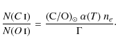
|
(5) |
Using (C/O)
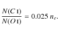
|
(6) |
Note that for
These values, in combination with n(C
I), indicate a
larger ionisation fraction towards Sk -67![]() 111 and LH 54-425.
111 and LH 54-425.
7 Conclusions
We
have presented UV absorption line measurements of Galactic H2,
C I, N I,
O I, Al II,
Si II, P II,
S III, Ar I,
and Fe II towards the six LMC stars
Sk -67![]() 111,
LH 54-425, Sk -67
111,
LH 54-425, Sk -67![]() 107, Sk -67
107, Sk -67![]() 106,
Sk -67
106,
Sk -67![]() 104,
and Sk -67
104,
and Sk -67![]() 101,
and analysed the properties of the Galactic disc gas in these lines of
sight. Our sight-lines were chosen within
101,
and analysed the properties of the Galactic disc gas in these lines of
sight. Our sight-lines were chosen within ![]() in RA, with an almost constant Dec, to allow us to investigate the
small-scale structures of the interstellar gas within
<1.5 pc (assuming that the foreground gas exists at a
distance of <1 kpc), with the smallest separation
corresponding to <0.08 pc. For four of the sight-lines,
Sk -67
in RA, with an almost constant Dec, to allow us to investigate the
small-scale structures of the interstellar gas within
<1.5 pc (assuming that the foreground gas exists at a
distance of <1 kpc), with the smallest separation
corresponding to <0.08 pc. For four of the sight-lines,
Sk -67![]() 101,
Sk -67
101,
Sk -67![]() 104,
Sk -67
104,
Sk -67![]() 106,
and Sk -67
106,
and Sk -67![]() 107,
we also analysed STIS spectral data, from which we have further
determined the column densities of C I*, C I**,
Mg II, Si IV,
S II, Mn II,
and Ni II. The STIS data provide
additional absorption lines for some of the species already available
in the FUSE spectra, allowing us to have a more reliable determination
of the column densities.
107,
we also analysed STIS spectral data, from which we have further
determined the column densities of C I*, C I**,
Mg II, Si IV,
S II, Mn II,
and Ni II. The STIS data provide
additional absorption lines for some of the species already available
in the FUSE spectra, allowing us to have a more reliable determination
of the column densities.
In the spectral range of FUSE we are able to gain information
from the different excitation levels of H2,
which provides us with valuable information about the fine structure of
the gas, because H2 arises in the coolest
regions of the interstellar clouds, and enables us to derive the
physical properties of the gas. The H2
absorptions show considerable variation between our sight-lines. The
lines of sight to Sk -67![]() 101 and Sk -67
101 and Sk -67![]() 104 contain a
significantly higher amount of H2, about
2 dex in their column densities, compared to Sk -67
104 contain a
significantly higher amount of H2, about
2 dex in their column densities, compared to Sk -67![]() 111. The
rotational excitation of H2 towards
Sk -67
111. The
rotational excitation of H2 towards
Sk -67![]() 101
to Sk -67
101
to Sk -67![]() 107
agrees with a core-envelope structure of the H2
gas with an average temperature of
107
agrees with a core-envelope structure of the H2
gas with an average temperature of ![]() K,
typical for CNM. This, and the low Doppler parameter of the lower J-levels,
indicates that the molecular hydrogen probably arises in confined dense
regions in these sight-lines, where it is self-shielded from
UV-radiation. The gas to LH 54-425 and Sk -67
K,
typical for CNM. This, and the low Doppler parameter of the lower J-levels,
indicates that the molecular hydrogen probably arises in confined dense
regions in these sight-lines, where it is self-shielded from
UV-radiation. The gas to LH 54-425 and Sk -67![]() 111, on the
other hand, appears to be fully thermalised, with
111, on the
other hand, appears to be fully thermalised, with ![]() K.
This could suggest that within the <
K.
This could suggest that within the <
![]() ,
we sample a core of a molecular hydrogen cloud, and reach the edge
between Sk -67
,
we sample a core of a molecular hydrogen cloud, and reach the edge
between Sk -67![]() 107
and Sk -67
107
and Sk -67![]() 111.
After including the LH 54-425 sight-line in our study,
however, the spatial variation is not a smooth change from
Sk -67
111.
After including the LH 54-425 sight-line in our study,
however, the spatial variation is not a smooth change from
Sk -67![]() 101
to Sk -67
101
to Sk -67![]() 111
(Fig. 8),
and density fluctuation on scales smaller than the extent of 5
111
(Fig. 8),
and density fluctuation on scales smaller than the extent of 5![]() cannot be excluded.
cannot be excluded.
In order to trace these variations back to the actual density
variations and changes in the physical properties of the gas we have
derived the densities partly based on the formation-dissociation
equilibrium of molecular hydrogen using the measured H2
and O I column densities, and
partly based on the excitation of the fine-structure levels of neutral
carbon. For the latter we have also used the derived ![]() (H2),
assuming that C I and H2
exist in the same physical region. The density derived in this way is
(H2),
assuming that C I and H2
exist in the same physical region. The density derived in this way is ![]() towards Sk -67
towards Sk -67![]() 101
to Sk -67
101
to Sk -67![]() 107,
for which we have relatively accurate measurements for column densities
of C I and C I*,
as well as
107,
for which we have relatively accurate measurements for column densities
of C I and C I*,
as well as ![]() .
This is well above the value
.
This is well above the value ![]() derived based on a formation-dissociation equilibrium of H2.
This is most likely because the available hydrogen for molecular
formation is less than the total Galactic
derived based on a formation-dissociation equilibrium of H2.
This is most likely because the available hydrogen for molecular
formation is less than the total Galactic ![]() derived from N(O I) along a line of sight.
Moreover, the H2 self-shielding could be
overestimated (and thus
derived from N(O I) along a line of sight.
Moreover, the H2 self-shielding could be
overestimated (and thus ![]() underestimated) because of a complex absorber geometry. Thus that value
for
underestimated) because of a complex absorber geometry. Thus that value
for ![]() gives a minimum density required for the existence of the H2.
gives a minimum density required for the existence of the H2.
On all sight-lines ![]() . If we assume that
. If we assume that ![]() is proportional to
is proportional to ![]() (from C I) in the same way as for the inner
region of a molecular cloud (meaning
(from C I) in the same way as for the inner
region of a molecular cloud (meaning ![]() ),
we can derive from Eq. (2) the column density of H I
that coexists with H2 in FDE. We so find that
this is 18% of the total
),
we can derive from Eq. (2) the column density of H I
that coexists with H2 in FDE. We so find that
this is 18% of the total ![]() (averaged over the sight-lines Sk -67
(averaged over the sight-lines Sk -67![]() 101 to Sk -67
101 to Sk -67![]() 107). It is
of course likely that the partly molecular core is more dense because
it is confined, and
107). It is
of course likely that the partly molecular core is more dense because
it is confined, and ![]() not linearly related to the
not linearly related to the ![]() as assumed above. Furthermore,
as assumed above. Furthermore, ![]() as derived from C I is the averaged density
of the molecular part of the gas, where C I
exists, and again not related to all the H I
gas along a line of sight as assumed above. Thus, the
as derived from C I is the averaged density
of the molecular part of the gas, where C I
exists, and again not related to all the H I
gas along a line of sight as assumed above. Thus, the ![]() together with the
together with the ![]() give only an upper limit for the pathlength of the partly molecular
cloud to be
give only an upper limit for the pathlength of the partly molecular
cloud to be ![]() pc
(included in Table 5).
These derived pathlengths are of the same size as (or smaller than) our
lateral extent of the sight-lines (<1.5 pc). This
derived upper limit for
pc
(included in Table 5).
These derived pathlengths are of the same size as (or smaller than) our
lateral extent of the sight-lines (<1.5 pc). This
derived upper limit for ![]() also agrees with the higher density ratio for the LH 54-425
sight-line, derived in Sect. 6.1, which
otherwise is difficult to explain if we consider this sight-line to
sample the edge of the same cloud with the core on the Sk -67
also agrees with the higher density ratio for the LH 54-425
sight-line, derived in Sect. 6.1, which
otherwise is difficult to explain if we consider this sight-line to
sample the edge of the same cloud with the core on the Sk -67![]() 101 to
Sk -67
101 to
Sk -67![]() 107
sight-lines. Based on
107
sight-lines. Based on ![]() and an average density of
and an average density of ![]() ,
,
![]() in
the direction of LH 54-425 and Sk -67
in
the direction of LH 54-425 and Sk -67![]() 111 is
estimated to be 0.1 and 0.6 pc, respectively. Given these
small sizes, the H2 patches observed on these
six lines of sight are not necessarily connected. The small pathlength
is further important for the shielding of the molecular gas, given the
small amount of H I that is possibly
available in FDE with H2.
111 is
estimated to be 0.1 and 0.6 pc, respectively. Given these
small sizes, the H2 patches observed on these
six lines of sight are not necessarily connected. The small pathlength
is further important for the shielding of the molecular gas, given the
small amount of H I that is possibly
available in FDE with H2.
We thus conclude that the H2 observed
along these six lines of sight exists in rather small cloudlets with an
upper size ![]() ,
and possibly even less, <0.1 pc, as implied by the
LH 54-425 sight-line. Part of the absorbing gas is possibly
located at a distance closer than the 1 kpc assumed thus far,
resulting in an even smaller spatial scale. This agrees with the sub-pc
structure of molecular clouds previously detected by e.g., Pan et al. (2001), Lauroesch et al. (2000),
Richter
et al. (2003b,a), and Marggraf et al. (2004).
On a smaller scale of 5 to 104 AU however, Boissé et al. (2009)
found no variation in the column density of the H2,
observed over a period of almost five years towards the Galactic
high-velocity star HD 34078. This despite the variations in
the CH column densities found over the same period. They concluded that
while the variation in CH and CH+ is due to the
chemical structure of a gas that is in interaction with the star, the H2,
located in a quiescent gas unaffected by the star, remains
homogeneously distributed. Hence no small-scale density structure was
proposed in the quiescent gas within this scale.
Our spatial resolution limits us to the smallest separation
of 17
,
and possibly even less, <0.1 pc, as implied by the
LH 54-425 sight-line. Part of the absorbing gas is possibly
located at a distance closer than the 1 kpc assumed thus far,
resulting in an even smaller spatial scale. This agrees with the sub-pc
structure of molecular clouds previously detected by e.g., Pan et al. (2001), Lauroesch et al. (2000),
Richter
et al. (2003b,a), and Marggraf et al. (2004).
On a smaller scale of 5 to 104 AU however, Boissé et al. (2009)
found no variation in the column density of the H2,
observed over a period of almost five years towards the Galactic
high-velocity star HD 34078. This despite the variations in
the CH column densities found over the same period. They concluded that
while the variation in CH and CH+ is due to the
chemical structure of a gas that is in interaction with the star, the H2,
located in a quiescent gas unaffected by the star, remains
homogeneously distributed. Hence no small-scale density structure was
proposed in the quiescent gas within this scale.
Our spatial resolution limits us to the smallest separation
of 17
![]() .
We have therefore no further information about the AU-scale structure
of the molecular gas in these lines of sight.
.
We have therefore no further information about the AU-scale structure
of the molecular gas in these lines of sight.
The absorber pathlength through the disc has previously been
found to be divided into smaller cloudlets of H I-absorbers
(Welty et al. 1999),
which are not necessarily physically connected to the cloud with the
observed H2. While the clumpy nature of H2
is verified by different studies, the Galactic H I gas,
when sampled over a line of sight, normally does not show variations on
small scales, since such effects statistically cancel out and smooth
the total observed H I (or O I
in our case). If such cloudlets exist in the Galactic disc component,
their radial velocity should be similar, and therefore would not be
resolved in our spectra. Our derived density ratio ![]() ,
as well as the relative abundances, suggest that the number of these
absorbers might differ along the sight-lines, being less towards
LH 54-425 and Sk -67
,
as well as the relative abundances, suggest that the number of these
absorbers might differ along the sight-lines, being less towards
LH 54-425 and Sk -67![]() 111. This interpretation also
agrees with the higher electron density derived for these lines of
sight.
111. This interpretation also
agrees with the higher electron density derived for these lines of
sight.
We summarised in Sect. 1 the detection of small-scale structure by different independent methods. This paper presents yet another approach to identify the structure of the gas on small scales. FUV and UV spectral data, with the large range of transitions particularly of H2 and O I together with the fine-structure of C I, provide a sensitive approach to study the physical properties of the gas on small scales. However, our spatial resolution is limited to the separation of our background sources, and does not allow us to directly detect the fine structure that might exist on even smaller scales. Our findings are consistent with the small-scale structure found earlier in the interstellar medium, and suggest inhomogeneity in the interstellar Galactic gas down to, and possibly below, scales of 0.1 pc.
We thank Ole Marggraf for his careful proofreading of this paper. SNS was supported through grant BO779/30 by the German Research Foundation (DFG).
References
- Abgrall, H., Roueff, E., Launay, F., Roncin, J. Y., & Subtil, J. L. 1993a, A&AS, 101, 273 [Google Scholar]
- Abgrall, H., Roueff, E., Launay, F., Roncin, J. Y., & Subtil, J. L. 1993b, A&AS, 101, 323 [Google Scholar]
- Andrews, S. M., Meyer, D. M., & Lauroesch, J. T. 2001, ApJ, 552, L73 [NASA ADS] [CrossRef] [Google Scholar]
- Asplund, M., Grevesse, N., & Sauval, A. J. 2005, ASPC, 336, 25 [Google Scholar]
- Bates, B., Catney, M. G., & Keenan, F. P. 1990, MNRAS, 245, 238 [NASA ADS] [Google Scholar]
- Bates, B., Gilheany, S., & Wood, K. D. 1991, MNRAS, 252, 600 [NASA ADS] [Google Scholar]
- Bates, B., Shaw, C. R., Kemp, S. N., Keenan, F. P., & Davies, R. D. 1995, ApJ, 444, 672 [NASA ADS] [CrossRef] [Google Scholar]
- Boissé, P., Rollinde, E., Hily-Blant, P., et al. 2009, A&A, 501, 221 [NASA ADS] [CrossRef] [EDP Sciences] [Google Scholar]
- Clifton, T. R., Frail, D. A., Kulkarni, S. R., & Weisberg, J. M. 1988, ApJ, 333, 332 [NASA ADS] [CrossRef] [Google Scholar]
- Cohen, J. G. 1978, ApJ, 223, 487 [NASA ADS] [CrossRef] [Google Scholar]
- Danforth, C. W., Howk, J. C., Fullerton, A. W., Blair, W. P., & Sembach, K. R. 2002, ApJS, 139, 81 [NASA ADS] [CrossRef] [Google Scholar]
- de Boer, K. S., & Morton, D. C. 1974, A&A, 37, 305 [NASA ADS] [Google Scholar]
- de Boer, K. S., Koppenaal, K., & Pottasch, S. R. 1973, A&A, 28, 145 [NASA ADS] [Google Scholar]
- de Boer, K. S., Richter, P., Bomans, D. J., Heithausen, A., & Koornneef, J. 1998, A&A, 338, L5 [NASA ADS] [Google Scholar]
- Dieter, N. H., Welch, W. J., & Romney, J. D. 1976, ApJ, 206, L113 [NASA ADS] [CrossRef] [Google Scholar]
- Draine, B. T. 1998, ApJ, 509, L41 [NASA ADS] [CrossRef] [Google Scholar]
- Draine, B. T., & Bertoldi, F. 1996, ApJ, 468, 269 [NASA ADS] [CrossRef] [EDP Sciences] [Google Scholar]
- Elmegreen, B. G. 1997, ApJ, 480, 674 [NASA ADS] [CrossRef] [Google Scholar]
- Faison, M. D., & Goss, W. M. 2001, AJ, 121, 2706 [NASA ADS] [CrossRef] [Google Scholar]
- Frail, D. A., Weisberg, J. M., Cordes, J. M., & Mathers, C. 1994, ApJ, 436, 144 [NASA ADS] [CrossRef] [Google Scholar]
- Heiles, C. 1997, ApJ, 481, 193 [NASA ADS] [CrossRef] [Google Scholar]
- Jenkins, E. B., Oegerle, W. R., Gry, C., et al. 2000, ApJ, 538, L81 [NASA ADS] [CrossRef] [MathSciNet] [Google Scholar]
- Lauroesch, J. T., & Meyer, D. M. 2003, ApJ, 591, L123 [NASA ADS] [CrossRef] [Google Scholar]
- Lauroesch, J. T., Meyer, D. M., & Blades, J. C. 2000, ApJ, 543, L43 [CrossRef] [Google Scholar]
- Marggraf, O. 2004, Ph.D. Thesis, Rheinischen Friedrich-Wilhelms-Universität Bonn [Google Scholar]
- Marggraf, O., Bluhm, H., & de Boer, K. S. 2004, A&A, 416, 251 [NASA ADS] [CrossRef] [EDP Sciences] [Google Scholar]
- McClure-Griffiths, N. M., Pisano, D. J., Calabretta, M. R., et al. 2009, ApJS, 181, 398 [NASA ADS] [CrossRef] [Google Scholar]
- Meyer, D. M. 1990, ApJ, 364, L5 [NASA ADS] [CrossRef] [Google Scholar]
- Meyer, D. M., & Lauroesch, J. T. 1999, ApJ, 520, L103 [NASA ADS] [CrossRef] [Google Scholar]
- Moos, H. W., Cash, W. C., Cowie, L. L., et al. 2000, ApJ, 538, L1 [NASA ADS] [CrossRef] [Google Scholar]
- Moos, H. W., Sembach, K. R., Vidal-Madjar, A., et al. 2002, ApJS, 140, 3 [NASA ADS] [CrossRef] [Google Scholar]
- Morton, D. C. 2003, ApJS, 149, 205 [NASA ADS] [CrossRef] [MathSciNet] [Google Scholar]
- Pan, K., Federman, S. R., & Welty, D. E. 2001, ApJ, 558, L105 [NASA ADS] [CrossRef] [Google Scholar]
- Péquignot, D., & Aldrovandi, S. M. V. 1986, A&A, 161, 169 [NASA ADS] [Google Scholar]
- Richter, P. 2000, A&A, 359, 1111 [NASA ADS] [Google Scholar]
- Richter, P., Widmann, H., de Boer, K. S., et al. 1998, A&A, 338, L9 [NASA ADS] [Google Scholar]
- Richter, P., Sembach, K. R., & Howk, J. C. 2003a, A&A, 405, 1013 [NASA ADS] [CrossRef] [EDP Sciences] [Google Scholar]
- Richter, P., Wakker, B. P., Savage, B. D., & Sembach, K. R. 2003b, ApJ, 586, 230 [NASA ADS] [CrossRef] [Google Scholar]
- Sahnow, D. J., Moos, H. W., Ake, T. B., et al. 2000, ApJ, 538, L7 [NASA ADS] [CrossRef] [Google Scholar]
- Savage, B. D., & de Boer, K. S. 1981, ApJ, 243, 460 [NASA ADS] [CrossRef] [Google Scholar]
- Sofia, U. J., & Jenkins, E. B. 1998, ApJ, 499, 951 [NASA ADS] [CrossRef] [Google Scholar]
- Spitzer, L. 1978, Physical processes in the interstellar medium (New York: Wiley-Interscience) [Google Scholar]
- Spitzer, L. J., & Cochran, W. D. 1973, ApJ, 186, L23 [NASA ADS] [CrossRef] [Google Scholar]
- Spitzer, L. J., & Zweibel, E. G. 1974, ApJ, 191, L127 [NASA ADS] [CrossRef] [Google Scholar]
- Walker, M., & Wardle, M. 1998, ApJ, 498, L125 [NASA ADS] [CrossRef] [Google Scholar]
- Wardle, M., & Walker, M. 1999, ApJ, 527, L109 [NASA ADS] [CrossRef] [PubMed] [Google Scholar]
- Watson, J. K., & Meyer, D. M. 1996, ApJ, 473, L127 [NASA ADS] [CrossRef] [Google Scholar]
- Welty, D. E. 2007, ApJ, 668, 1012 [NASA ADS] [CrossRef] [Google Scholar]
- Welty, D. E., & Fitzpatrick, E. L. 2001, ApJ, 551, L175 [NASA ADS] [CrossRef] [Google Scholar]
- Welty, D. E., Frisch, P. C., Sonneborn, G., & York, D. G. 1999, ApJ, 512, 636 [NASA ADS] [CrossRef] [Google Scholar]
Footnotes
- ... MASTa
- Multi-Mission Archive at Space Telescope: http://archive.stsci.edu/
- ... errorsb
- Based on 68
 of the data points having a residual within
  from the corresponding COG coefficient.
- ... densitiesc
- The fit has been including all possible b>2 km s-1.
All Tables
Table 1: Information about the FUSE data as retrieved from the MAST archive.
Table 2: S/N per resolution element measured within a few Ångström around the listed wavelength.
Table 3:
Column densities ![]() (N in cm-2) of Galactic
foreground gas, 1
(N in cm-2) of Galactic
foreground gas, 1![]() errors, and Doppler parameter b [km s-1]
measured from the COGa.
errors, and Doppler parameter b [km s-1]
measured from the COGa.
Table 4: List of absorption lines, used for the column density determination in one or more sight-linesa.
Table 5: Physical conditions in the Milky Way foreground gas as derived from the data.
All Figures
|
|
Figure 1:
H |
| Open with DEXTER | |
| In the text | |
|
|
Figure 2: O I absorption at 936.63 (from FUSE:SiC), 1039.23 (from FUSE:LiF), and 1302.17 Å (from STIS) and the continuum fit is shown for all six stars (names given at right). The solid line is the continuum fit to which the spectrum has been normalised, the dashed lines show the upper and lower continuum choice. The bars at the top mark the known absorption component velocities for the O I lines (see Sect. 3.1). |
| Open with DEXTER | |
| In the text | |
|
|
Figure 3:
Logarithmic column densities of H2 and
O I towards Sk -67 |
| Open with DEXTER | |
| In the text | |
|
|
Figure 4:
Sample of H2 absorption lines from different
excited levels shown for the different sight-lines. The sight-lines are
labelled on the right, from top to bottom:
Sk -67 |
| Open with DEXTER | |
| In the text | |
|
|
Figure 5:
Rotational excitation of H2 in foreground
Galactic disc gas. For each sight-line the column density (cm-2)
of H2 in level J is
divided by the statistical weight gJ
and plotted on a logarithmic scale against the excitation energy EJ.
The corresponding Boltzmann temperatures are given with the fitted
lines. This temperature is represented by a straight line through the
three lowest rotational states J=0, 1,
and 2. The higher J-levels indicate the
level of UV-pumping. For Sk -67 |
| Open with DEXTER | |
| In the text | |
|
|
Figure 6:
Sample of COGs of O I
for the six sight-lines (the star name on top of each figure). Each
plot shows C OGs for b=1,3,6,7,8 km s-1.
The solid line is the resulting COG from the
best fit (b=7 km s-1),
and the dotted lines (b=6 and b=8 km s-1)
correspond to approximately |
| Open with DEXTER | |
| In the text | |
|
|
Figure 7:
Metal abundances plotted against the angular separation. The abundances
are expressed as the ratio |
| Open with DEXTER | |
| In the text | |
|
|
Figure 8:
Density ratio, |
| Open with DEXTER | |
| In the text | |
Copyright ESO 2010
Current usage metrics show cumulative count of Article Views (full-text article views including HTML views, PDF and ePub downloads, according to the available data) and Abstracts Views on Vision4Press platform.
Data correspond to usage on the plateform after 2015. The current usage metrics is available 48-96 hours after online publication and is updated daily on week days.
Initial download of the metrics may take a while.