| Issue |
A&A
Volume 510, February 2010
|
|
|---|---|---|
| Article Number | A80 | |
| Number of page(s) | 14 | |
| Section | Interstellar and circumstellar matter | |
| DOI | https://doi.org/10.1051/0004-6361/200913310 | |
| Published online | 16 February 2010 | |
The ISO Long Wavelength Spectrometer line spectrum of VY Canis Majoris and other oxygen-rich evolved stars![[*]](/icons/foot_motif.png)
E. T. Polehampton1,2,3,![]() - K. M. Menten1 - F. F. S. van der Tak4,1 - G. J. White2,5
- K. M. Menten1 - F. F. S. van der Tak4,1 - G. J. White2,5
1 - Max-Planck-Institut für Radioastronomie, Auf dem Hügel 69, 53121 Bonn, Germany
2 - Space Science & Technology Department, Rutherford Appleton Laboratory, Chilton, Didcot, Oxfordshire, OX11 0QX, UK
3 - Department of Physics, University of Lethbridge, 4401 University Drive, Lethbridge, Alberta, T1J 1B1, Canada
4 - Netherlands Institute for Space Research (SRON), Landleven 12, 9747 AD Groningen, The Netherlands
5 - Department of Physics and Astronomy, The Open University, Milton Keynes, MK6 7AA, UK
Received 16 September 2009 / Accepted 10 November 2009
Abstract
Context. The far-infrared spectra of circumstellar envelopes
around various oxygen-rich stars were observed using the ISO Long
Wavelength Spectrometer (LWS). These have been shown to be spectrally
rich, particularly in water lines, indicating a high H2O abundance.
Aims. We have examined high signal-to-noise ISO LWS observations
of the luminous supergiant star, VY CMa, with the aim of
identifying all of the spectral lines. By paying particular attention
to water lines, we aim to separate the lines due to other species, in
particular, to prepare for forthcoming observations that will cover the
same spectral range using Herschel PACS and at higher spectral
resolution using Herschel HIFI and SOFIA.
Methods. We have developed a fitting method to account for
blended water lines using a simple weighting scheme to distribute the
flux. We have used this fit to separate lines due to other species
which cannot be assigned to water. We have applied this approach to
several other stars which we compare with VY CMa.
Results. We present line fluxes for the unblended H2O and CO lines, and present detections of several possible ![]() vibrationally excited water lines. We also identify blended lines of OH, one unblended and several blended lines of NH3, and one possible detection of H3O+.
vibrationally excited water lines. We also identify blended lines of OH, one unblended and several blended lines of NH3, and one possible detection of H3O+.
Conclusions. The spectrum of VY CMa shows a detection
of emission from virtually every water line up to 2000 K above the
ground state, as well as many additional higher energy and some
vibrationally excited lines. A simple rotation diagram analysis shows
large scatter (probably due to some optically thick lines). The fit
gives a rotational temperature of 670
+210-130 K, and lower limit on the water column density of
![]() cm-2. We estimate a CO column density
cm-2. We estimate a CO column density ![]() 100 times
lower, showing that water is the dominant oxygen carrier. The other
stars that we examined have similar rotation temperatures, but their H2O column densities are an order of magnitude lower (as are the mass loss rates).
100 times
lower, showing that water is the dominant oxygen carrier. The other
stars that we examined have similar rotation temperatures, but their H2O column densities are an order of magnitude lower (as are the mass loss rates).
Key words: stars: AGB and post-AGB - stars: individual: VY Canis Majoris - supergiants - circumstellar matter
1 Introduction
Circumstellar envelopes form around red giant and supergiant stars during the later stages of their evolution. The mass loss from the stars results in an expanding envelope of material consisting of dust and molecules whose absorption and/or emission can be observed from infrared through radio wavelengths. In oxygen-rich stars with high mass loss rates, the cooling of the envelope is believed to be dominated by rotational lines from water (H2O) vapour (e.g. Justtanont et al. 1994), which has a rich far infrared (FIR) spectrum. The FIR range also contains the rotational transitions of other simple molecules and molecular ions.
The Infrared Space Observatory (ISO; Kessler et al. 1996) satellite has revolutionised the study of circumstellar envelopes by allowing access to all the spectral features in the mid- and far-infrared range. ISO spectra observed using the Short Wavelength Spectrometer (SWS; de Graaw et al. 1996) and Long Wavelength Spectrometer (LWS; Clegg et al. 1996) have previously been analysed, showing that the majority of the detected features in the FIR range are due to the rotational transitions of water (W Hya SWS: Neufeld et al. 1996; W Hya LWS: Barlow et al. 1996; R Cas LWS: Truong-Bach et al. 1999; VY CMa SWS: Neufeld et al. 1999).
Table 1: Characteristics of the stars used in this paper.
In this paper, we present a dataset containing the ISO LWS spectra of
the red supergiant star VY CMa, and several other evolved
stars. The basic parameters of these spectra, such as identifications
of lines over the wavelength range 45-![]() m
and their fluxes are discussed here. We concentrate on the results from
VY CMa, as it shows the spectrum with the highest signal to
noise ratio and the line identifications are typical of several other
stars in the sample. The SWS line spectrum for this star has previously
been presented by
Neufeld et al. (1999). The continuum emission of the SWS and LWS spectra has been modeled by Harwit et al. (2001) and the LWS line emission has
been briefly described by Barlow (1999). VY CMa is thought to be in a late stage of stellar evolution, and appears extremely bright at
infrared wavelengths. It has a mass loss rate estimated to be of the order of
m
and their fluxes are discussed here. We concentrate on the results from
VY CMa, as it shows the spectrum with the highest signal to
noise ratio and the line identifications are typical of several other
stars in the sample. The SWS line spectrum for this star has previously
been presented by
Neufeld et al. (1999). The continuum emission of the SWS and LWS spectra has been modeled by Harwit et al. (2001) and the LWS line emission has
been briefly described by Barlow (1999). VY CMa is thought to be in a late stage of stellar evolution, and appears extremely bright at
infrared wavelengths. It has a mass loss rate estimated to be of the order of
![]() to
to
![]()
![]() yr-1 with a period of higher mass loss in the past (Decin et al. 2006). It is located at the edge of a molecular cloud (Lada & Reid 1978), and has a distance derived from H2O and SiO masers of
yr-1 with a period of higher mass loss in the past (Decin et al. 2006). It is located at the edge of a molecular cloud (Lada & Reid 1978), and has a distance derived from H2O and SiO masers of ![]() 1.1 kpc from the Sun
(Choi et al. 2008; Reid & Menten, in preparation). In Sect. 3,
we estimate the column densities of water and CO in the envelope of
VY CMa to determine which is the dominant oxygen carrier. In
Sect. 4, we compare the
results from VY CMa with several other stars that were also
observed with the ISO LWS. The characteristics of these stars are shown
in Table 1.
1.1 kpc from the Sun
(Choi et al. 2008; Reid & Menten, in preparation). In Sect. 3,
we estimate the column densities of water and CO in the envelope of
VY CMa to determine which is the dominant oxygen carrier. In
Sect. 4, we compare the
results from VY CMa with several other stars that were also
observed with the ISO LWS. The characteristics of these stars are shown
in Table 1.
Table 2: Log of the L01 observations used in this paper.
![\begin{figure}
\par\includegraphics[width=15.5cm,clip]{13310fg1.eps}
\end{figure}](/articles/aa/full_html/2010/02/aa13310-09/img21.png)
|
Figure 1:
LWS spectra (45-197 |
| Open with DEXTER | |
2 Observations and data reduction
A complete set of uniformly processed LWS grating spectra (using ISO
observing mode L01) have been uploaded to the ISO Data Archive![]() as highly processed data products (HPDP; Lloyd et al. 2003).
This allows us to make a detailed comparison of consistently and
accurately calibrated spectral lines observed toward a sample of
different stars. The objects, positions and ISO target dedicated
time (TDT) numbers of the data we have used are shown in
Table 2.
as highly processed data products (HPDP; Lloyd et al. 2003).
This allows us to make a detailed comparison of consistently and
accurately calibrated spectral lines observed toward a sample of
different stars. The objects, positions and ISO target dedicated
time (TDT) numbers of the data we have used are shown in
Table 2.
To check the accuracy of the standard HPDP pipeline processing for our individual objects, we downloaded and manually reduced the LWS L01 spectrum of VY CMa, comparing it with the HPDP data (to examine the effects of automatically removing glitches and dark current subtraction). Both the test observations and the HPDP were initially processed with the LWS off line pipeline (OLP) version 10.
In order to reduce the data by hand, we used the LWS Interactive Analysis (LIA; Lim et al. 2002) software to optimise the dark current subtraction for each LWS detector. The absolute responsivity correction was not adjusted interactively because the OLP data already contains a better method of calculating the corrections to that available in the LIA software. Glitches were carefully removed from each scan by hand using the ISO Spectral Analysis Package (ISAP; Sturm et al. 1998). In addition, forward and backward scans were compared and the regions where one direction was affected by the response time of the detectors were removed (this can occur when the grating was scanned in the direction of increasing detector response from the edge of each band). A correction for fringing was applied using the LWS defringing algorithm within ISAP. The forward and reverse scans for each detector were then averaged.
A careful comparison of the interactively reduced and HPDP spectra showed that there were only minor differences in the final strength of the lines. This is mainly due to the defringing step which was only performed in the HPDP processing for detectors that the pipeline judged significantly affected (in the case of VY CMa, only for detector SW5, whereas interactively we judged defringing to make most difference to detector LW4). Further differences that may cause problems are that in the HPDP data reduction, both scan directions were simply averaged together (without accounting for the transient response of the detectors) and deglitching was carried out automatically. However, neither of these appear to have led to the introduction of spurious features in the HPDP spectrum.
The largest difference between the two data reduction
techniques is an improvement in the spectral shape of data from
detector SW1 in the HPDP data. This is due to an additional correction
in the HPDP pipeline that removes a double-peaked structure (with peaks
at ![]() 45
45 ![]() m and
m and ![]() 48
48 ![]() m) that is believed to be due to spurious features in the SW1 relative spectral response function (Lloyd et al. 2003).
Using this correction allows us to have much greater confidence in the
spectral shape observed using SW1 between 43 and 50
m) that is believed to be due to spurious features in the SW1 relative spectral response function (Lloyd et al. 2003).
Using this correction allows us to have much greater confidence in the
spectral shape observed using SW1 between 43 and 50 ![]() m.
m.
In conclusion, we determined that the HPDP pipeline did not introduce
spurious artifacts that could be mistaken for lines, and that it had
superior calibration for detector SW1. Therefore, we have used
only the HPDP data for all of the stars in our sample. We applied
multiplicative shifts to individual detector data to align their
continua by examining the overlap region between pairs of detectors.
However, this was not important for the spectrum of VY CMa
because the absolute flux calibration applied by the HPDP already gave
very good agreement between adjacent detectors, with the only exception
being SW1, which had an absolute flux ![]() 20% higher than SW2. For the other stars, the shifts were more often required for the long wavelength detectors (up to
20% higher than SW2. For the other stars, the shifts were more often required for the long wavelength detectors (up to ![]() 30%).
In order to examine the line fluxes, we subtracted the continuum level
by fitting a 3rd order polynomial baseline to the data from each
detector independently.
30%).
In order to examine the line fluxes, we subtracted the continuum level
by fitting a 3rd order polynomial baseline to the data from each
detector independently.
Several well known spurious features that resemble lines remain
in the spectra, and these are labeled in the plots presented here (e.g.
features in absorption at 77 ![]() m using SW5 and 191
m using SW5 and 191 ![]() m using LW5, and features in emission at 107
m using LW5, and features in emission at 107 ![]() m and 109
m and 109 ![]() m
using LW2; Grundy, private communication). Some of these lines occur in
the overlap region between two detectors and so can be ignored by
selecting the optimum wavelength ranges to use. To provide a further
check that the line features we have identified are real, we compared
the spectra to observations of the asteroid Ceres, which
should not contain any spectral line features (but does contain the
spurious features).
m
using LW2; Grundy, private communication). Some of these lines occur in
the overlap region between two detectors and so can be ignored by
selecting the optimum wavelength ranges to use. To provide a further
check that the line features we have identified are real, we compared
the spectra to observations of the asteroid Ceres, which
should not contain any spectral line features (but does contain the
spurious features).
Where there were multiple LWS observations of the sample stars that showed good agreement, these were co-added to increase the signal to noise ratio. This applied to IRC+10011 and RX Boo (see Table 2). Although several other observations were also available for R Cas (TDTs 26300712, 56801715 and 56801552), we have used only the one with longest integration time (TDT 56801440).
The LWS beam size was ![]() 80'', and the spectral resolution was 0.29
80'', and the spectral resolution was 0.29 ![]() m for detectors SW1-SW5 and 0.6
m for detectors SW1-SW5 and 0.6 ![]() m for detectors LW1-LW5 (Gry et al. 2003). The RMS noise in the spectra varies for the different stars, but is roughly (10-20)
m for detectors LW1-LW5 (Gry et al. 2003). The RMS noise in the spectra varies for the different stars, but is roughly (10-20)
![]() W cm-2
W cm-2 ![]() m-1 in the short wavelength detectors (measured between 87 and 89.5
m-1 in the short wavelength detectors (measured between 87 and 89.5 ![]() m), and (0.5-2.2)
m), and (0.5-2.2)
![]() W cm-2
W cm-2 ![]() m-1 in the long wavelength detectors (measured between 140 and 142
m-1 in the long wavelength detectors (measured between 140 and 142 ![]() m). The wavelength bin width is 0.04
m). The wavelength bin width is 0.04 ![]() m for the short wavelength detectors and 0.13
m for the short wavelength detectors and 0.13 ![]() m for the long wavelength detectors. The final spectra before continuum subtraction are shown in Fig. 1, plotted as
m for the long wavelength detectors. The final spectra before continuum subtraction are shown in Fig. 1, plotted as
![]() .
In this figure, the spectra have been smoothed with a window of 5 wavelength bins.
.
In this figure, the spectra have been smoothed with a window of 5 wavelength bins.
3 Results: VY CMa
In this paper we concentrate on identifying and characterising the spectral lines in the LWS data between 45 and 196 ![]() m. The following sections present the line identifications for VY CMa in this range.
m. The following sections present the line identifications for VY CMa in this range.
![\begin{figure}
\par\includegraphics[angle=0,width=14cm,clip]{13310fg2.ps}
\end{figure}](/articles/aa/full_html/2010/02/aa13310-09/img23.png)
|
Figure 2: Continuum subtracted LWS spectrum of VY CMa with all water line transitions with upper levels up to 2000 K above the ground state marked below the spectrum (para: lower, ortho: upper of the two groups) and other lines marked individually above the spectrum. |
| Open with DEXTER | |
![\begin{figure}
\par\includegraphics[angle=0,width=13.5cm,clip]{13310fg3.eps}
\end{figure}](/articles/aa/full_html/2010/02/aa13310-09/img24.png)
|
Figure 3:
An example of our water line fit for VY CMa for the region 59-68 |
| Open with DEXTER | |
3.1 Water
The SWS spectrum of VY CMa has already been shown to be rich in the rotational lines of water (Neufeld et al. 1999). They identified at least 41 features due to water in the spectral range 29.5-45 ![]() m,
with transitions up to 2939 K above the ground state. Many of the
remaining weak features in the SWS spectrum can also be explained by
including higher energy transitions of water. Here, we have analysed
the LWS spectrum and carefully checked all of the prominent emission
features. This shows that most of the detected lines can be attributed
to rotational transitions in the vibrational ground state of water.
m,
with transitions up to 2939 K above the ground state. Many of the
remaining weak features in the SWS spectrum can also be explained by
including higher energy transitions of water. Here, we have analysed
the LWS spectrum and carefully checked all of the prominent emission
features. This shows that most of the detected lines can be attributed
to rotational transitions in the vibrational ground state of water.
The LWS spectra after continuum subtraction are shown in Fig. 2.
The LWS spectral resolution is lower than achieved with the SWS, and
many of the features are blended together. However, at longer
wavelengths there are at least some gaps with few or no water lines in
at all, giving the possibility to uniquely identify several other
molecular species. The continuum level was estimated individually for
each detector by fitting a 3rd order polynomial through the lowest
points in the spectrum as described in Sect. 2. For wavelengths greater than ![]() 80
80 ![]() m,
there are sufficient gaps between emission features, and this method
should give a reasonable estimate of the continuum. However, severe
line blending occurs <
m,
there are sufficient gaps between emission features, and this method
should give a reasonable estimate of the continuum. However, severe
line blending occurs <![]() m,
and in this region the continuum level may have been overestimated
because there is insufficiently clear space between the lines. This
means that the line fluxes may be systematically underestimated.
However, the fluxes for lines at wavelengths <
m,
and in this region the continuum level may have been overestimated
because there is insufficiently clear space between the lines. This
means that the line fluxes may be systematically underestimated.
However, the fluxes for lines at wavelengths <![]() m
are unlikely to be underestimated by more than a factor of a few,
because sufficient contamination of the continuum would require very
strong emission from lines lying >2000 K above the ground state
and corresponding emission >80
m
are unlikely to be underestimated by more than a factor of a few,
because sufficient contamination of the continuum would require very
strong emission from lines lying >2000 K above the ground state
and corresponding emission >80 ![]() m is not seen.
m is not seen.
In Fig. 2, all
the central wavelengths of all rotational ortho- and para- water
transitions in its vibrational ground state are marked for energies up
to 2000 K. Virtually every one of these transitions is matched by
a feature in the data. This upper state energy is not a fundamental
limit on the features detected in the spectrum, but adopted to ease of
viewing the labels displayed at the LWS spectral resolution. The
inclusion of lines with higher upper state energy levels suggests that
many of the low lying lines are probably blended with other water
features. Several spectral regions that are free of lines from
transitions with energies below 2000 K clearly show that higher
energy transitions are present. These wavelengths are individually
marked in Fig. 2 (particularly 68-70 ![]() m and 152-156
m and 152-156 ![]() m).
m).
3.2 Fitting the water lines
In this section, we describe fitting the water lines in the vibrational
ground state. Due to the large number of blended lines in the spectrum,
any determination of the flux of individual lines is likely to be
rather uncertain. In addition, there will be systematic errors
introduced in the line fluxes due to the uncertainty in the underlying
continuum level at the shortest wavelengths. In order to estimate the
line fluxes, we have used a method that simultaneously fits the water
lines in the vibrational ground state up to a certain energy level
(upper state energy less than 2000 K above ground). The best fit
is found by increasing the flux density at each line centre until the
model reaches the data. The line wavelengths are fixed at their
catalogue values (taken from the JPL line catalogue; Pickett et al. 1998), and line widths fixed at the spectral resolution of the ISO detectors (0.29 ![]() m for LWS detectors SW1-SW5 and 0.6
m for LWS detectors SW1-SW5 and 0.6 ![]() m for detectors LW1-LW5; Gry et al. 2003). Lines occuring within the wavelength range of each of the 10 LWS detectors are fitted together.
m for detectors LW1-LW5; Gry et al. 2003). Lines occuring within the wavelength range of each of the 10 LWS detectors are fitted together.
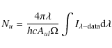
The flux densities at the centres of all lines measured by the detector
are increased by a step that is weighted (for each line) relative to
the Einstein coefficient for spontaneous emission, Aul, (with values taken from the JPL catalogue; Pickett et al. 1998), and
![]() ,
where Eu/k is the energy of the upper state above ground in K, and
,
where Eu/k is the energy of the upper state above ground in K, and
![]() is a single temperature applied to all lines. This ensures that lines
with higher weight are given preference in blends. However, it does not
necessarily mean that the final flux will be distributed following the
weights - the actual shape of the data may allow a line with a lower
weight to have a higher flux than one with a high weight. The weighting
scheme does not treat ortho and para lines separately. The basic step
size in the model is set to 0.01 times flux density at the wavelength
of the strongest line, and the individual step for all other lines are
multiplied by their weights,
is a single temperature applied to all lines. This ensures that lines
with higher weight are given preference in blends. However, it does not
necessarily mean that the final flux will be distributed following the
weights - the actual shape of the data may allow a line with a lower
weight to have a higher flux than one with a high weight. The weighting
scheme does not treat ortho and para lines separately. The basic step
size in the model is set to 0.01 times flux density at the wavelength
of the strongest line, and the individual step for all other lines are
multiplied by their weights,

|
(1) |
where
![\begin{displaymath}
w_{\lambda}=\frac{A_{ul}}{{\rm {MAX}}[A_{ul}]}\frac{{\rm {ex...
..._{\rm weight})}{{\rm {MAX}}[{{\exp}}(-E_{u}/kT_{\rm weight})]}
\end{displaymath}](/articles/aa/full_html/2010/02/aa13310-09/img31.png)
and s is the basic step size, defined by,
![\begin{displaymath}s = \frac{{\rm {MAX}}[I_{\lambda-{\rm data}}]}{100}
\end{displaymath}](/articles/aa/full_html/2010/02/aa13310-09/img32.png)
|
(3) |
where the operation MAX finds the maximum value over the lines occuring within the wavelength range of the particular LWS detector being fitted.
A first estimate for the value of
![]() to use in this weighting function was determined from a rotation diagram (see Sect. 3.3) using a fit weighted relative to Aul only,
to use in this weighting function was determined from a rotation diagram (see Sect. 3.3) using a fit weighted relative to Aul only,
![\begin{displaymath}
w_{\lambda}=\frac{A_{ul}}{{\rm {MAX}}[A_{ul}]}.
\end{displaymath}](/articles/aa/full_html/2010/02/aa13310-09/img33.png)
Figure 3 shows a fairly representative example of the final fit, for the region 59-68
The advantage of this technique to estimate the line fluxes is that
it is much faster than carrying out a multiple Gaussian ![]() fit. Moreover, the flux in complicated blends is not overestimated (as
it could be in a free Gaussian fit if the line shape is affected by
other species). The disadvantage is that it takes no account of the
overall excitation of the molecule, except within blends where the
lines are explicitly weighted according to Aul and
fit. Moreover, the flux in complicated blends is not overestimated (as
it could be in a free Gaussian fit if the line shape is affected by
other species). The disadvantage is that it takes no account of the
overall excitation of the molecule, except within blends where the
lines are explicitly weighted according to Aul and
![]() .
The final errors on each line flux are highly correlated in the various
blended groups and therefore difficult to rigorously estimate. However,
this fitting method provides a good starting point to investigate the
spectrum, and represents the best that can be achieved using data
observed with the available spectral resolution.
.
The final errors on each line flux are highly correlated in the various
blended groups and therefore difficult to rigorously estimate. However,
this fitting method provides a good starting point to investigate the
spectrum, and represents the best that can be achieved using data
observed with the available spectral resolution.
In order to check the reliability of the automatic fitting
routine, we compared the fit using several different weighting schemes:
no weight, weighted relative to Aul only (Eq. (4)), and weighted relative to Aul and exp
![]() (Eq. (2)).
For the few completely unblended lines, we also carried out a manual
fit using ISAP and in general this agrees within the errors with the
automatic procedure. The unblended line fluxes for these different fit
methods are shown for VY CMa and IK Tau in
Table 4. We estimate that the fitting errors for unblended lines are 15-20%.
(Eq. (2)).
For the few completely unblended lines, we also carried out a manual
fit using ISAP and in general this agrees within the errors with the
automatic procedure. The unblended line fluxes for these different fit
methods are shown for VY CMa and IK Tau in
Table 4. We estimate that the fitting errors for unblended lines are 15-20%.
The final line fluxes determined from the fit for all lines up to 2000 K above the ground state (including blends) are shown in Table A.1, for all of the stars investigated. In order to check the blended fits, we have compared our results for R Cas with those obtained by Truong-Bach et al. (1999). Our fitted values are in reasonable agreement (in a line by line comparison, many fluxes agree to better than 50%, and the remaining discrepencies can be explained by the fact that we have included more blends). We estimate that our blended line fluxes are probably of the correct order of magnitude (unless the assumptions used for the weighting scheme within the fit are wildly incorrect).
We have also checked our fitted fluxes with the analysis of Maercker et al. (2008) who fitted water lines in a similar sample of stars. In general at long wavelengths where the lines are well separated, we find very good agreement in fitted fluxes. However, the difference in our analysis is that we have included the possibility of blends with higher energy lines. This is clearly necessary in VY CMa to account for all of the detected features. In the analysis of Maercker et al. (2008), they sometimes calculated model values lower than their quoted line fits to the data. This may be partly due to not identifying blends - some of our fitted fluxes which include blends (where Maercker et al. did not include a blend) give values closer to their model predictions. On the other hand, in some cases, our simple treatment that includes many blended lines seems to underestimate the flux compared to their model, suggesting that we may have not distributed the flux correctly. However, this comparison shows that in these stars, it is very important to consider that detected features may be due to blends of water transitions over a very wide range in energy, and it is not enough to merely consider the (strongest) lower level lines.
3.3 Excitation of H2O
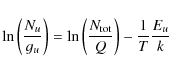
In order to investigate the fitted line fluxes, we have used a simple rotation diagram approach (e.g. Goldsmith & Langer 1999).
Assuming that all transitions are in local thermodynamic equilibrium
(LTE), there is a linear relationship between the natural logarithm of
the upper state column density per statistical weight and the energy
above the ground state (i.e. following the Boltzmann distribution),
|
(5) |
where Nu is the column density in the upper state, gu is the statistical weight of the upper state,
|
(6) |
where
![\begin{figure}
\par\includegraphics[width=8.8cm,clip]{13310fg4.eps}
\end{figure}](/articles/aa/full_html/2010/02/aa13310-09/img42.png)
|
Figure 4: Rotation diagram resulting from fit to water lines in the LWS spectrum of VY CMa weighted by Aul and Eu. Ortho water lines are shown as filled circles and para water lines as crosses. The best fit to lines with upper state energies less than 2000 K (ignoring outlying points) is shown, giving a rotational temperature of 670 +210-130 K. |
| Open with DEXTER | |
Figure 4 shows the rotation diagram for VY CMa. Even though we know that this model does not accurately describe reality (VY CMa actually has a very complex environment - see Sect. 5), and many of the lines are likely to be optically thick and/or subthermally excited, we think it provides an instructive starting point to view the fitted fluxes, particularly since the number of lines that we are fitting is very large (141 lines used in the fit). The lower energy lines in Fig. 4 (<1500 K) are unlikely to be completely optically thin, and Maercker et al. (2008) found that the water lines in their sample of stars were generally subthermally excited (although more thermalised in IK Tau than the other stars they looked at).
Although most of the results cluster along a straight line, there is a large scatter. This is exactly the effect we should expect to see for a nonlinear molecule which has a mixture of optically thick and thin lines that are not necessarily in LTE (Goldsmith & Langer 1999, see their Figs. 5 and 8). The lines least likely to be optically thick are those with upper state energies above 1500 K, although these lines are more likely to be blended, and so have large fitting errors.
Taking into account the above uncertainties, the fitted value
for the total column density should be taken as a lower limit, and the
temperature as a very rough estimate of the actual kinetic temperature
(also bearing in mind that we expect a range of different thermal
environments). The best fit straight line has a slope corresponding to
a rotational temperature of
![]() K
(the error was derived only taking into account the scatter in the data
points). There does not appear to be a significant difference between
the ortho- and para- lines. Due to the challenges described earlier
regarding accurate flux estimation, we have discounted far outlying
points by carrying out a 2
K
(the error was derived only taking into account the scatter in the data
points). There does not appear to be a significant difference between
the ortho- and para- lines. Due to the challenges described earlier
regarding accurate flux estimation, we have discounted far outlying
points by carrying out a 2![]() clip. These points, which can lie far above the best fit line, could be
due to miss-fitting the flux of lines in blends. The rest of the
scatter is due to real departures from the simple model as described
above. More detailed modelling, beyond the scope of this paper is
required to investigate these effects. The isotopic lines of H218O
could be used to investigate the optical depths, but this will require
future higher resolution observations (a useful limit on the H218O emission is difficult with the current LWS data).
clip. These points, which can lie far above the best fit line, could be
due to miss-fitting the flux of lines in blends. The rest of the
scatter is due to real departures from the simple model as described
above. More detailed modelling, beyond the scope of this paper is
required to investigate these effects. The isotopic lines of H218O
could be used to investigate the optical depths, but this will require
future higher resolution observations (a useful limit on the H218O emission is difficult with the current LWS data).
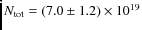
The best fit intercept point gives
![]() cm-2. The partition function at 300 K is given in the JPL catalogue (Pickett et al. 1998) as 178.12. The value scales as T1.5 which leads to a partition function of 594.47 at 670 K, and this gives a lower limit on the total water column density of
cm-2. The partition function at 300 K is given in the JPL catalogue (Pickett et al. 1998) as 178.12. The value scales as T1.5 which leads to a partition function of 594.47 at 670 K, and this gives a lower limit on the total water column density of
![]() cm-2.
cm-2.
3.4 Vibrationally excited water
In addition to transitions from the vibrational ground state of water, Neufeld et al. (1999) also identified 4 features with water in its vibrationally excited
![]() state. Rotational transitions of water in its
state. Rotational transitions of water in its
![]() state have also been observed at millimetre and submillimetre
wavelengths, showing that the emission probably comes from a region
close to the star (Menten & Melnick 1989; Menten et al. 2006).
At the spectral resolution of the LWS grating, vibrationally excited
water is much harder to separate. However, in the longer wavelength
detectors there are three features that match with wavelengths of
state have also been observed at millimetre and submillimetre
wavelengths, showing that the emission probably comes from a region
close to the star (Menten & Melnick 1989; Menten et al. 2006).
At the spectral resolution of the LWS grating, vibrationally excited
water is much harder to separate. However, in the longer wavelength
detectors there are three features that match with wavelengths of
![]() rotational transitions. These are shown in Table 3.
It is possible that other vibrationally excited lines exist in the
spectrum but all other transitions with similar energies occur in
blends. Also, the ground state transitions were identified first, which
may mean that some vibrationally excited lines could have been
misidentified as ground state ones (for example, the
rotational transitions. These are shown in Table 3.
It is possible that other vibrationally excited lines exist in the
spectrum but all other transitions with similar energies occur in
blends. Also, the ground state transitions were identified first, which
may mean that some vibrationally excited lines could have been
misidentified as ground state ones (for example, the
![]() 212-101 line occurs at 170.928
212-101 line occurs at 170.928 ![]() m, close to the feature we have labelled as
15511-16214 in Fig. 2). Higher spectral resolution observations would be required to unambiguously identify all of the vibrationally excited lines.
m, close to the feature we have labelled as
15511-16214 in Fig. 2). Higher spectral resolution observations would be required to unambiguously identify all of the vibrationally excited lines.
Table 3:
Possible rotational lines from the vibrationally excited
![]() state of water in the LWS spectrum of VY CMa.
state of water in the LWS spectrum of VY CMa.
Menten et al. (2006) detected two transitions of vibrationally excited water using the 12 m Atacama Pathfinder Experiment telescope (APEX): 523-616 at 336.2 GHz and 661-752 at 293.6 GHz. They used a model to calculate the optical depths and intensities of their measured lines, assuming that the transitions were thermalised. We have applied the same model to calculate the optical depth and predicted flux of our three detected FIR transitions. The line wavelengths and transition parameters were taken from the JPL line catalogue (Pickett et al. 1998). If we make the same assumptions about the emitting region (T = 1000 K, thermalised lines, uniform region within 0.05'' from the star) and assume a line width of 20 km s-1 (the same as the APEX lines), we derive high optical depths of 500, 270 and 600 for the three lines in Table 3. The predicted fluxes are a few 10-21 W cm-2, which underestimate our measured LWS fluxes by factors of 36-86.
The model predictions were closer for the sub-millimetre lines observed by Menten et al. (2006), underestimating their measured intensities by only a factor of 2.3 and 5, and a factor of 3 for the 550-643 232.6 GHz transition observed by Menten & Melnick (1989). The underestimated intensity was explained by the fact that the 294 GHz line may be boosted by weak maser action.
Table 4: Fitted fluxes for the unblended lines in the spectrum of VY CMa and IK Tau.
We have also applied the model to the SWS lines observed by Neufeld et al. (1999), predicting that the SWS lines should be stronger than the LWS lines, which is not observed. The SWS fluxes measured by Neufeld et al. (1999) are reproduced by the model within factors of 2-8. The optical depths for the SWS lines are predicted to be in the order of 104.
The model seems to be much worse at predicting the FIR fluxes than
those in the sub-millimetre and mid-infrared. At the high optical
depths predicted, the only parameters in the model that affect the
final fluxes are the temperature of the emitting region, the line width
and assumed source size. The flux calculated by the model could be
brought into better agreement by a combination of increasing the
temperature and size of the emitting region, as the line fluxes are ![]() linearly
proportional to both. However, increasing the assumed emission region
size has a large effect on the predicted sub-mm main beam brightness
temperatures. The excitation temperature does not have a large impact
on the sub-mm lines, but a much higher temperature would be needed than
is indicated by previous measurements (see Menten et al. 2006).
linearly
proportional to both. However, increasing the assumed emission region
size has a large effect on the predicted sub-mm main beam brightness
temperatures. The excitation temperature does not have a large impact
on the sub-mm lines, but a much higher temperature would be needed than
is indicated by previous measurements (see Menten et al. 2006).
This either indicates that there is another problem with the simple model (for example, different excitation conditions for the FIR lines) or that the measured LWS fluxes are overestimated (possibly due to additional line blending which has not been taken into account here). Observations at higher spectral resolution are needed to confirm the fluxes, and more detailed modelling is required, taking into account both the sub-mm and infrared lines.
3.5 CO lines
In the LWS spectrum of VY CMa, the water line density decreases toward the longer wavelengths. CO is known to be an abundant molecule in O-rich circumstellar envelopes and many observations have been made via its millimetre and sub-millimetre transitions (e.g. Decin et al. 2006; Ziurys et al. 2009; Kemper et al. 2003). The lowest energy CO transition in the ISO spectral range is J = 14-13, with upper state energy of 580 K above the ground state.
Several CO lines have previously been reported in the LWS spectral range toward R Cas (Truong-Bach et al. 1999) and W Hya (Barlow et al. 1996). In addition gaseous CO absorption has been observed around 4.5 ![]() m in the SWS spectra of O-rich stars (e.g. Sylvester et al. 1997).
m in the SWS spectra of O-rich stars (e.g. Sylvester et al. 1997).
In the LWS spectrum of VY CMa, we observe some contribution to the spectrum from all CO lines from J = 14-13 up to J = 25-24. These lines are labeled in Fig. 2. The higher energy lines are difficult to identify due to blending with water lines and the best detection is of the lowest energy lines which are generally well separated. The fluxes of these lines at long wavelengths were determined in two ways and are shown in Table 5. As a first estimate, the CO fluxes were determined by fitting the excess emission after subtracting the water line fit described in Sect. 3.2. The flux was also determined by a manual Gaussian fit using ISAP, taking account of nearby blended lines with a multi-Gaussian fit. The automatic fit generally underestimates the flux compared to the manual fit, probably because water was given preference in the blends for the automatic fit (although the automatic fit is within the errors of the ISAP fit). The true flux is probably between the two values.
We have carried out a rotation diagram analysis of the CO fluxes in the same way as described in Sect. 3.3 for H2O. This is shown in Fig. 5, with a fit to the 4 lowest energy lines (the fit ignores the fluxes for J=19-18 and J=21-20
which have very large error bars). This gives a rough estimate of the
rotational temperature and total column density as we are only fitting
a few lines. However, the results should be more reliable than for H2O, because the high excitation CO lines are likely to be optically thin. We have used the manual ISAP fluxes from Table 5 and fitted a straight line weighted by their errors. This gives
![]() K and
K and
![]() cm-2. The partition function at 300 K is given in the JPL catalogue (Pickett et al. 1998) as 108.865, and this leads to a total CO column density of
cm-2. The partition function at 300 K is given in the JPL catalogue (Pickett et al. 1998) as 108.865, and this leads to a total CO column density of
![]() cm-2.
cm-2.
![\begin{figure}
\par\includegraphics[width=8.8cm,clip]{13310fg5.eps}
\vspace*{-2mm}
\end{figure}](/articles/aa/full_html/2010/02/aa13310-09/img65.png)
|
Figure 5: Rotation diagram for the CO lines observed towards VY CMa. The dashed line is a fit to the 4 lowest energy lines using the manually fitted fluxes from Table 5. |
| Open with DEXTER | |
This column density is approximately 100 times lower than the H2O column density calculated in Sect. 3.3, showing that generally in the VY CMa envelope, water is the dominant oxygen carrier (although the H2O and CO come from different temperature regions).
Table 5:
Fitted fluxes for the CO lines observed above 120 ![]() m for VY CMa.
m for VY CMa.
3.6 Other lines: OH, NH and HO+
Several other lines were detected in the spectrum of VY CMa. These are summarised in Table 6 and described in the following paragraphs.
We detect strong emission from OH at 163 ![]() m, which is blended with the CO J = 16-15 line. This line is due to the lowest energy pure rotational transition in the
m, which is blended with the CO J = 16-15 line. This line is due to the lowest energy pure rotational transition in the
![]() ladder of OH. Some contribution from the next transition in this ladder at 99
ladder of OH. Some contribution from the next transition in this ladder at 99 ![]() m
is probably also detected. In addition we detect emission in several
other transitions of OH such as the lowest rotational line in the
m
is probably also detected. In addition we detect emission in several
other transitions of OH such as the lowest rotational line in the
![]() ladder at 119
ladder at 119 ![]() m. As the cross ladder transition at 34
m. As the cross ladder transition at 34 ![]() m is seen in absorption in the SWS spectrum (Neufeld et al. 1999),
we might also expect the other cross ladder transitions in the LWS
range to be in absorption (e.g. the other transitions from the
m is seen in absorption in the SWS spectrum (Neufeld et al. 1999),
we might also expect the other cross ladder transitions in the LWS
range to be in absorption (e.g. the other transitions from the
![]() J =3/2 level at 53
J =3/2 level at 53 ![]() m and 79
m and 79 ![]() m). However, these are both blended with water emission.
m). However, these are both blended with water emission.
The FIR lines of ammonia in its ![]() bending-inversion mode are rotation-inversion transitions, with the lowest energy transition K = 2, J = 3-2 at 165.60 and 169.97
bending-inversion mode are rotation-inversion transitions, with the lowest energy transition K = 2, J = 3-2 at 165.60 and 169.97 ![]() m. There is a clear emission peak at 165.60
m. There is a clear emission peak at 165.60 ![]() m in the spectrum of VY CMa (see Fig. 2).
This does not overlap with any water lines and has a width comparable
to the instrument resolution. We think that the assignment of this
feature to NH3 is secure because it does not appear to be
blended. There are only a few other species that could provide
alternative explanations for the line: the most likely two choices are
HNC J = 20-19 and H3O+ K = 0, J = 5-4. The HNC line has a high energy upper level at 913 K and the corresponding transition in HCN at 161.35
m in the spectrum of VY CMa (see Fig. 2).
This does not overlap with any water lines and has a width comparable
to the instrument resolution. We think that the assignment of this
feature to NH3 is secure because it does not appear to be
blended. There are only a few other species that could provide
alternative explanations for the line: the most likely two choices are
HNC J = 20-19 and H3O+ K = 0, J = 5-4. The HNC line has a high energy upper level at 913 K and the corresponding transition in HCN at 161.35 ![]() m is not clearly detected. If the line was due to H3O+,
there should have been other features present which are not observed.
The line is also observed in the spectrum of IK Tau (see
Sect. 4).
m is not clearly detected. If the line was due to H3O+,
there should have been other features present which are not observed.
The line is also observed in the spectrum of IK Tau (see
Sect. 4).
The NH3 line at 169.97 ![]() m occurs in a blend with water lines. The transition at the next highest energy in NH3 is K = 3, J = 4-3 at 124.65 and 127.11
m occurs in a blend with water lines. The transition at the next highest energy in NH3 is K = 3, J = 4-3 at 124.65 and 127.11 ![]() m. Both these lines occur in the wing of water emission (but are marked in Fig. 2).
m. Both these lines occur in the wing of water emission (but are marked in Fig. 2).
Ammonia has been observed in the envelopes of both carbon and oxygen
rich stars - the first detection in an O-rich envelope was made by McLaren & Betz (1980) in VY CMa, VX Sgr and IRC+10420. They observed several vibration-rotation transitions in the ![]() band at 10.5 and 10.7
band at 10.5 and 10.7 ![]() m. Subsequently these transitions have been measured in more detail for VY CMa by Monnier et al. (2000) and references therein. These observations show that NH3 probably forms near the termination of the gas acceleration phase.
m. Subsequently these transitions have been measured in more detail for VY CMa by Monnier et al. (2000) and references therein. These observations show that NH3 probably forms near the termination of the gas acceleration phase.
The only detection of the radio inversion transitions of ammonia in O-rich stars was made by Menten & Alcolea (1995) toward IK Tau and IRC+10420. They found that the strongest inversion transition for IK Tau was K = 3, J =3-3 whereas for IRC+10420 was K = 1, J = 1-1. This implies that with a higher mass loss rate, photodissociation occurs further from the star and the NH3 emission comes from a lower temperature region.
The H3O+ ion has a similar pyramidal structure to the isoelectronic molecule NH3. In an analogous way to NH3,
the oxygen atom can tunnel through the plane of the molecule leading to
an inversion splitting of the rotational levels. However, for H3O+, the inversion splitting is very large (55.34 cm-1 for the ![]() bending-inversion mode; Liu et al. 1986).
This means that the pure inversion transitions occur at FIR wavelengths
rather than in the radio regime as for ammonia. Several
rotation-inversion transitions at 1 mm have previously been
detected in giant molecular clouds (Phillips et al. 1992; Wootten et al. 1991) and the lines near 300 GHz mapped toward Sgr B2 (van der Tak et al. 2006). Several of the FIR transitions have also been observed in absorption toward Sgr B2 with ISO (Goicoechea & Cernicharo 2001; Polehampton et al. 2007).
bending-inversion mode; Liu et al. 1986).
This means that the pure inversion transitions occur at FIR wavelengths
rather than in the radio regime as for ammonia. Several
rotation-inversion transitions at 1 mm have previously been
detected in giant molecular clouds (Phillips et al. 1992; Wootten et al. 1991) and the lines near 300 GHz mapped toward Sgr B2 (van der Tak et al. 2006). Several of the FIR transitions have also been observed in absorption toward Sgr B2 with ISO (Goicoechea & Cernicharo 2001; Polehampton et al. 2007).
Table 6: Summary of other lines detected in the VY CMa spectrum.
The peak abundance of H3O+ in oxygen-rich circumstellar envelopes is predicted to be ![]() 10-7 (Mamon et al. 1987), with the major formation route being the photodissociation of H2O
and OH. Excitation is probably via the absorption of mid-IR radiation
rather than collisions and thus absorption bands may also be observable
at 10 and 17
10-7 (Mamon et al. 1987), with the major formation route being the photodissociation of H2O
and OH. Excitation is probably via the absorption of mid-IR radiation
rather than collisions and thus absorption bands may also be observable
at 10 and 17 ![]() m. The only (possible) detection of H3O+ toward an evolved star so far is the 2
m. The only (possible) detection of H3O+ toward an evolved star so far is the 2![]() feature observed toward VY CMa by Phillips et al. (1992) at the correct velocity for the K = 0 J =3-2 396 GHz transition.
feature observed toward VY CMa by Phillips et al. (1992) at the correct velocity for the K = 0 J =3-2 396 GHz transition.
In the LWS grating spectrum of VY CMa, the spectral
resolution is low and the inversion and rotation-inversion transitions
are difficult to separate from the water lines. However, there is an
unidentified feature at the correct wavelength for the K = 1 J =2-2 transition at 183.68 ![]() m. The other low energy inversion transition may contribute to the (water) emission features around 180-181
m. The other low energy inversion transition may contribute to the (water) emission features around 180-181 ![]() m.
The rotation-inversion transitions are harder to positively identify as
they occur at shorter wavelengths where the density of water lines is
higher.
m.
The rotation-inversion transitions are harder to positively identify as
they occur at shorter wavelengths where the density of water lines is
higher.
In several O-rich star spectra, a feature at 157.8 ![]() m has been assigned to the atomic fine structure line of ionised carbon at 157.74
m has been assigned to the atomic fine structure line of ionised carbon at 157.74 ![]() m (Truong-Bach et al. 1999; Sylvester et al. 1997). This line also appears in the VY CMa spectrum but no other atomic lines are clearly visible. Sylvester et al. (1997)
attribute this line to bad subtraction of the galactic background in
their sources. However, at least some contribution to it can be
explained by the 955-862 para water line at 157.88
m (Truong-Bach et al. 1999; Sylvester et al. 1997). This line also appears in the VY CMa spectrum but no other atomic lines are clearly visible. Sylvester et al. (1997)
attribute this line to bad subtraction of the galactic background in
their sources. However, at least some contribution to it can be
explained by the 955-862 para water line at 157.88 ![]() m.
The upper level for this transition occurs 2031 K above the ground
state. In VY CMa there could be some contribution from both
lines.
m.
The upper level for this transition occurs 2031 K above the ground
state. In VY CMa there could be some contribution from both
lines.
There are several remaining unassigned features in the spectrum and these are labeled as ``U-lines'' in Fig. 2. In addition, there are several species which have transitions in the range and are predicted to be reasonably abundant in O-rich circumstellar envelopes, but are not possible to detect due to line blending with water (e.g. HCN, H2S; Willacy & Millar 1997).
![\begin{figure}
\par\resizebox{14.5cm}{!}{\includegraphics[angle=0]{13310f6a.eps}}\par\resizebox{14.5cm}{!}{\includegraphics[angle=0]{13310f6b.eps}}
\end{figure}](/articles/aa/full_html/2010/02/aa13310-09/img75.png)
|
Figure 6: Comparison of the spectrum of VY CMa with the other stars (the spectra of the other stars have been smoothed and shifted for clarity - see text). |
| Open with DEXTER | |
4 Comparison with other stars
The spectrum of the oxygen rich Mira variable IK Tau shows
remarkable similarity to that of VY CMa. However, the line
fluxes shown in Fig. 6 are ![]() 4 times weaker and the continuum level
4 times weaker and the continuum level ![]() 10 times
lower. Since it was only observed for about twice the integration time
of VY CMa, the signal-to-noise of the spectrum appears lower
than that of VY CMa. Within the noise level and accuracy of
the continuum subtraction, all of the lines observed in the VY
CMa spectrum are present in the IK Tau spectrum,
generally with very similar relative intensities. Figure 6
shows the spectrum of IK Tau scaled by a factor of 4.5 and
compared to VY CMa. It is clear that the same lines are
detected in each object. There are, however, a few exceptions where
there are marked differences: there is much weaker OH emission with
respect to water in IK Tau. The OH line at 119
10 times
lower. Since it was only observed for about twice the integration time
of VY CMa, the signal-to-noise of the spectrum appears lower
than that of VY CMa. Within the noise level and accuracy of
the continuum subtraction, all of the lines observed in the VY
CMa spectrum are present in the IK Tau spectrum,
generally with very similar relative intensities. Figure 6
shows the spectrum of IK Tau scaled by a factor of 4.5 and
compared to VY CMa. It is clear that the same lines are
detected in each object. There are, however, a few exceptions where
there are marked differences: there is much weaker OH emission with
respect to water in IK Tau. The OH line at 119 ![]() m is not present and there may be less contribution to the 163
m is not present and there may be less contribution to the 163 ![]() m CO/OH blend from OH. Also the line at 99
m CO/OH blend from OH. Also the line at 99 ![]() m is weaker in IK Tau. However, the other lines such as CO, NH3 and the possible
m is weaker in IK Tau. However, the other lines such as CO, NH3 and the possible ![]() water lines are all present in both stars. In addition, the unidentified feature at 86
water lines are all present in both stars. In addition, the unidentified feature at 86 ![]() m
is present in both spectra. There is only one feature that is present
in IK Tau but not in VY CMa at 73.8
m
is present in both spectra. There is only one feature that is present
in IK Tau but not in VY CMa at 73.8 ![]() m.
m.
In Fig. 6, we also plot the other stars from Table 1. In order to compare the spectral lines, we have multiplied each continuum subtracted spectrum by factors of 4.5 for IK Tau and R Cas; 6 for TX Cam and 10 for RX Boo and IRC+10011. We have also smoothed the noisy spectra. Several key spectral lines are shown.
The other stars of a similar type to IK Tau (TX Cam, RX Boo, IRC+10011) have a much lower signal to noise ratio and their lines are weaker than IK Tau. However, the majority of detections in VY CMa and IK Tau also seem to be present in these stars.
We have fitted the water lines in the vibrational ground state for the other stars in the same way as for VY CMa and the results are shown in Table A.1. We have carried out a rotation diagram analysis for each star as described in Sect. 3.3, and the results are shown in Table 7, giving a rough estimate of the rotational temperature and a lower limit for the total water column density.
The rotational temperatures for the other stars are very similar
(within 25%) to the value found for VY CMa, which indicates
that the H2O-emitting gas is excited under similar conditions. If the excitation is dominated by collisions,
![]() should reflect the kinetic temperature of the gas because of the high
densities of AGB star envelopes. Alternatively, radiation may dominate
the excitation, in which case
should reflect the kinetic temperature of the gas because of the high
densities of AGB star envelopes. Alternatively, radiation may dominate
the excitation, in which case
![]() would reflect the temperature of the ambient radiation field. The only star where
would reflect the temperature of the ambient radiation field. The only star where
![]() deviates from the trend is IRC+10011, but in this case, the error on
deviates from the trend is IRC+10011, but in this case, the error on
![]() is rather large (due to a larger scatter in the data points in the rotation diagram).
is rather large (due to a larger scatter in the data points in the rotation diagram).
The derived H2O column densities for the other stars are lower than for VY CMa, with values ranging from 2% to 12% of the value for VY CMa. Since the other stars also have 10-100 times lower mass loss rates (see Table 1), this result indicates that water is also the main oxygen carrier in the other star envelopes. However, a direct scaling of N(H2O) with mass loss rate does not appear: the ratio of H2O column density and mass loss rate shows a large variation over our sample of stars (factor of >10).
Table 7: Results of fitting a straight line to the rotation diagram for all of the stars in our sample.
5 Summary
In this paper we present the ISO LWS spectrum of the luminous supergiant star VY CMa and give a brief description of the detected lines. We then compared the spectrum with several other evolved star spectra, particularly the Mira variable IK Tau.
The detected lines in the spectra of VY CMa and IK Tau are remarkably similar, both in the species detected and the relative intensity of the water lines.
We draw the following conclusions:
- We confirm that the spectra of our sample of evolved stars are
dominated by water line emission in the FIR, and we report the
detection of nearly all the H2O lines up to
 2000 K above the ground state.
- A simple rotation analysis of the water lines shows that there
are a probably a mixture of optically thick and thin lines which may be
subthermally excited (the fit gives a rotational temperature of 670
+210-130 K, and a corresponding column density
 cm-2 which should be treated a lower limit to the true value).
- We tentatively assign several of the detected features to excited water in its
 vibrational state.
- We estimate the column density of CO to be
 cm-2, showing that water is the dominant oxygen carrier in these envelopes.
- We present a detection of ammonia in VY CMa and IK Tau, and a tentative detection of the H3O+ ion toward VY CMa.
E. T. P. would like to thank E. Krügel for help and encouragement in Bonn, and also M. Barlow for helpful advice and T. W. Grundy for useful discussions about the ISO L01 spectra and HPDP data. We made use of the Cologne Database for Molecular Spectroscopy (CDMS; Müller et al. 2005). The LWS Interactive Analysis (LIA) package is a joint development of the ISO-LWS Instrument Team at the Rutherford Appleton Laboratory (RAL, UK - the PI Institute) and the Infrared Processing and Analysis Center (IPAC/Caltech, USA). The ISO Spectral Analysis Package (ISAP) is a joint development by the LWS and SWS Instrument Teams and Data Centres. Contributing institutes are CESR, IAS, IPAC, MPE, RAL and SRON.
Appendix A: Full list of fitted fluxes
Table A.1: All line fluxes calculated by our fitting procedure for the 6 stars.
References
- Barlow, M. J. 1999, in Asymptotic Giant Branch Stars, ed. T. Le Bertre, A. Lèbre, & C. Waelkens, IAU Symp., 191, 353 [Google Scholar]
- Barlow, M. J., Nguyen-Q-Rieu, Truong-Bach, et al. 1996, A&A, 315, L241 [NASA ADS] [Google Scholar]
- Choi, Y. K., Hirota, T., Honma, M., et al. 2008, PASJ, 60, 1007 [NASA ADS] [Google Scholar]
- Clegg, P. E., Ade, P. A. R., Armand, C., et al. 1996, A&A, 315, L38 [NASA ADS] [Google Scholar]
- de Graaw, T., Haser, L. N., Beintema, D. A., et al. 1996, A&A, 315, L49 [NASA ADS] [Google Scholar]
- Decin, L., Hony, S., de Koter, A., et al. 2006, A&A, 456, 549 [NASA ADS] [CrossRef] [EDP Sciences] [Google Scholar]
- Decin, L., Hony, S., de Koter, A., et al. 2007, A&A, 475, 233 [NASA ADS] [CrossRef] [EDP Sciences] [Google Scholar]
- Goicoechea, J. R., & Cernicharo, J. 2001, ApJ, 554, L213 [NASA ADS] [CrossRef] [Google Scholar]
- Goldsmith, P. F., & Langer, W. D. 1999, ApJ, 517, 209 [NASA ADS] [CrossRef] [Google Scholar]
- Gry, C., Swinyard, B., Harwood, A., et al. 2003, ISO Handbook Volume III (LWS), Version 2.1, ESA SAI-99-077/Dc [Google Scholar]
- Harwit, M., Malfait, K., Decin, L., et al. 2001, ApJ, 557, 844 [NASA ADS] [CrossRef] [Google Scholar]
- Justtanont, K., Skinner, C. J., & Tielens, A. G. G. M. 1994, ApJ, 435, 852 [NASA ADS] [CrossRef] [Google Scholar]
- Kemper, F., Stark, R., Justtanont, K., et al. 2003, A&A, 407, 609 [NASA ADS] [CrossRef] [EDP Sciences] [Google Scholar]
- Kessler, M. F., Steinz, J. A., Anderegg, M. E., et al. 1996, A&A, 315, L27 [NASA ADS] [Google Scholar]
- Lada, C. J., & Reid, M. J. 1978, ApJ, 219, 95 [NASA ADS] [CrossRef] [Google Scholar]
- Lim, T. L., Hutchinson, G., Sidher, S. D., et al. 2002, SPIE, 4847, 435 [NASA ADS] [CrossRef] [Google Scholar]
- Liu, D.-J., Oka, T., & Sears, T. J. 1986, J. Chem. Phys., 84, 1312 [NASA ADS] [CrossRef] [Google Scholar]
- Lloyd, C., Lerate, M. R., & Grundy, T. W. 2003, The LWS L01 Pipeline, version 1, available from the ISO Data Archive at http://www.iso.vilspa.esa.es/ida/ [Google Scholar]
- Maercker, M., Schöier, F. L., Olofsson, H., Bergman, P., & Ramstedt, S. 2008, A&A, 479, 779 [NASA ADS] [CrossRef] [EDP Sciences] [Google Scholar]
- Mamon, G. A., Glassgold, A. E., & Omont, A. 1987, ApJ, 323, 306 [NASA ADS] [CrossRef] [Google Scholar]
- McLaren, R. A., & Betz, A. L. 1980, ApJ, 240, L159 [NASA ADS] [CrossRef] [Google Scholar]
- Menten, K. M., & Alcolea, J. 1995, ApJ, 448, 416 [NASA ADS] [CrossRef] [Google Scholar]
- Menten, K. M., & Melnick, G. J. 1989, ApJ, 341, 91 [Google Scholar]
- Menten, K. M., Philipp, S. D., Güsten, R., et al. 2006, A&A, 454, L107 [NASA ADS] [CrossRef] [EDP Sciences] [Google Scholar]
- Menten, K. M., Lundgren, A., Belloche, A., Thorwirth, S., & Reid, M. 2008, A&A, 477, 185 [NASA ADS] [CrossRef] [EDP Sciences] [Google Scholar]
- Monnier, J. D., Danchi, W. C., Hale, D. S., Tuthill, P. G., & Townes, C. H. 2000, ApJ, 543, 868 [NASA ADS] [CrossRef] [Google Scholar]
- Müller, H. S. P., Schlöder, F., Stutzki, J., et al. 2005, J. Mol. Struct., 742, 215 [NASA ADS] [CrossRef] [Google Scholar]
- Muller, S., Dinh-V-Trung; Lim, J., Hirano, N., & Muthu, C., Kwok, S. 2007, ApJ, 656, 1109 [NASA ADS] [CrossRef] [Google Scholar]
- Neufeld, D. A., Chen, W., Melnick, G. J., et al. 1996, A&A, 315, L237 [NASA ADS] [Google Scholar]
- Neufeld, D. A., Feuchtgruber, H., Harwit, M., et al. 1999, ApJ, 517, L147 [Google Scholar]
- Olivier, E. A., Whitelock, P., & Marang, F. 2001, MNRAS, 326, 490 [NASA ADS] [CrossRef] [Google Scholar]
- Phillips, T. G., van Dishoeck, E. F., & Keene, J. 1992, ApJ, 399, 533 [NASA ADS] [CrossRef] [Google Scholar]
- Pickett, H. M., Poynter, R. L., Cohen, E. A., et al. 1998, J. Quant. Spectrosc. & Rad. Transfer, 60, 883 [Google Scholar]
- Polehampton, E. T., Baluteau, J.-P., Swinyard, B. M., et al. 2007, MNRAS, 377, 1122 [NASA ADS] [CrossRef] [Google Scholar]
- Smith, N., Hinkle, K., & Ryde, N. 2009, AJ, 137, 3558 [NASA ADS] [CrossRef] [Google Scholar]
- Sturm, E., Bauer, O. H., Lutz, D., et al. 1998, in Astronomical Data Analysis Software and Systems VII, ASP Conf. Ser., 145, 161 [Google Scholar]
- Sylvester, R. J., Barlow, M. J., Nguyen-Q-Rieu, et al. 1997, MNRAS, 291, L42 [NASA ADS] [CrossRef] [Google Scholar]
- Teyssier, D., Hernandez, R., Bujarrabal, V., Yoshida, H., & Phillips, T. G. 2006, A&A, 450, 167 [NASA ADS] [CrossRef] [EDP Sciences] [Google Scholar]
- Truong-Bach, Sylvester, R. J., Barlow, M. J., et al. 1999, A&A, 345, 925 [NASA ADS] [Google Scholar]
- van der Tak, F. F. S., Belloche, A., Schilke, P., et al. 2006, A&A, 454, L99 [NASA ADS] [CrossRef] [EDP Sciences] [Google Scholar]
- Willacy, K., & Millar, T. J. 1997, A&A, 324, 237 [NASA ADS] [Google Scholar]
- Wootten, A., Mangum, J. G., Turner, B. E., et al. 1991, ApJ, 380, L79 [NASA ADS] [CrossRef] [Google Scholar]
- Ziurys, L., Tenenbaum, E., Pulliam, R., Woolf, N., & Milam, S. 2009, ApJ, 695, 1604 [NASA ADS] [CrossRef] [Google Scholar]
Footnotes
- ... stars
- Based on observations with ISO, an ESA project with instruments funded by ESA Member States (especially the PI countries: France, Germany, the Netherlands and the United Kingdom) with the participation of ISAS and NASA.
- ...
- Current address: Space Science Department, Rutherford Appleton Laboratory, UK
- ... Archive
- See www.iso.esac.esa.int/ida/
All Tables
Table 1: Characteristics of the stars used in this paper.
Table 2: Log of the L01 observations used in this paper.
Table 3:
Possible rotational lines from the vibrationally excited
![]() state of water in the LWS spectrum of VY CMa.
state of water in the LWS spectrum of VY CMa.
Table 4: Fitted fluxes for the unblended lines in the spectrum of VY CMa and IK Tau.
Table 5:
Fitted fluxes for the CO lines observed above 120 ![]() m for VY CMa.
m for VY CMa.
Table 6: Summary of other lines detected in the VY CMa spectrum.
Table 7: Results of fitting a straight line to the rotation diagram for all of the stars in our sample.
Table A.1: All line fluxes calculated by our fitting procedure for the 6 stars.
All Figures
|
|
Figure 1:
LWS spectra (45-197 |
| Open with DEXTER | |
| In the text | |
|
|
Figure 2: Continuum subtracted LWS spectrum of VY CMa with all water line transitions with upper levels up to 2000 K above the ground state marked below the spectrum (para: lower, ortho: upper of the two groups) and other lines marked individually above the spectrum. |
| Open with DEXTER | |
| In the text | |
|
|
Figure 3:
An example of our water line fit for VY CMa for the region 59-68 |
| Open with DEXTER | |
| In the text | |
|
|
Figure 4: Rotation diagram resulting from fit to water lines in the LWS spectrum of VY CMa weighted by Aul and Eu. Ortho water lines are shown as filled circles and para water lines as crosses. The best fit to lines with upper state energies less than 2000 K (ignoring outlying points) is shown, giving a rotational temperature of 670 +210-130 K. |
| Open with DEXTER | |
| In the text | |
|
|
Figure 5: Rotation diagram for the CO lines observed towards VY CMa. The dashed line is a fit to the 4 lowest energy lines using the manually fitted fluxes from Table 5. |
| Open with DEXTER | |
| In the text | |
|
|
Figure 6: Comparison of the spectrum of VY CMa with the other stars (the spectra of the other stars have been smoothed and shifted for clarity - see text). |
| Open with DEXTER | |
| In the text | |
Copyright ESO 2010
Current usage metrics show cumulative count of Article Views (full-text article views including HTML views, PDF and ePub downloads, according to the available data) and Abstracts Views on Vision4Press platform.
Data correspond to usage on the plateform after 2015. The current usage metrics is available 48-96 hours after online publication and is updated daily on week days.
Initial download of the metrics may take a while.