| Issue |
A&A
Volume 510, February 2010
|
|
|---|---|---|
| Article Number | A56 | |
| Number of page(s) | 15 | |
| Section | Extragalactic astronomy | |
| DOI | https://doi.org/10.1051/0004-6361/200913229 | |
| Published online | 09 February 2010 | |
The [O III] emission line luminosity function of optically
selected type-2 AGN from zCOSMOS![[*]](/icons/foot_motif.png) ,
,
A. Bongiorno1,2 - M. Mignoli3 - G. Zamorani3 - F. Lamareille4 - G. Lanzuisi5,6 - T. Miyaji7,8 - M. Bolzonella3 - C. M. Carollo9 - T. Contini4 - J. P. Kneib10 - O. Le Fèvre10 - S. J. Lilly 9 - V. Mainieri11 - A. Renzini12 - M. Scodeggio13 - S. Bardelli3 - M. Brusa1 - K. Caputi9 - F. Civano5 - G. Coppa3,14 - O. Cucciati10 - S. de la Torre10,13,15 - L. de Ravel10 - P. Franzetti13 - B. Garilli13 - C. Halliday16 - G. Hasinger1,17 - A. M. Koekemoer18 - A. Iovino13 - P. Kampczyk9 - C. Knobel9 - K. Kovac9 - J. -F. Le Borgne4 - V. Le Brun10 - C. Maier9 - A. Merloni1,19 - P. Nair3 - R. Pello4 - Y. Peng9 - E. Perez Montero4,20 - E. Ricciardelli21 - M. Salvato17,19,22 - J. Silverman9 - M. Tanaka11 - L. Tasca10,13 - L. Tresse10 - D. Vergani3 - E. Zucca3 - U. Abbas10 - D. Bottini13 - A. Cappi3 - P. Cassata10,23 - A. Cimatti14 - L. Guzzo16 - A. Leauthaud10 - D. Maccagni13 - C. Marinoni24 - H. J. McCracken25 - P. Memeo13 - B. Meneux1 - P. Oesch9 - C. Porciani9 - L. Pozzetti3 - R. Scaramella26
1 - Max-Planck-Institut für extraterrestrische Physik (MPE), Giessenbachstraße 1, 85748 Garching bei München, Germany
2 -
University of Maryland, Baltimore County, 1000 Hilltop Circle, Baltimore, MD21250, USA
3 -
INAF-Osservatorio Astronomico di Bologna, via Ranzani 1, 40127 Bologna, Italy
4 -
Laboratoire d'Astrophysique de Toulouse-Tarbes, Université de Toulouse, CNRS, 14 avenue Edouard Belin, 31400 Toulouse, France
5 -
Harvard-Smithsonian Center for Astrophysics, 60 Garden Street, Cambridge, MA 02138, USA
6 -
Dipartimento di Fisica, Università di Roma La Sapienza, P.le A. Moro 2, 00185 Roma, Italy
7 - Instituto de Astronomía, Universidad Nacional Autónoma de
México, Ensenada, México, (mailing address: PO Box 439027,
San Ysidro, CA, 92143-9027, USA)
8 -
University of California, San Diego, Center for Astrophysics and Space Sciences, 9500 Gilman Drive, La Jolla, CA 92093-0424, USA
9 -
Department of Physics, ETH Zurich, 8093 Zurich, Switzerland
10 - Laboratoire d'Astrophysique de Marseille, CNRS-Université
d'Aix-Marseille, 38 rue Frédéric Joliot Curie, 13388 Marseille Cedex
13, France
11 -
ESO, Karl-Schwarzschild-Strasse 2, 85748 Garching bei München, Germany
12 -
INAF - Osservatorio Astronomico di Padova, Padova, Italy
13 -
INAF - Istituto di Astrofisica Spaziale e Fisica Cosmica di Milano, via Bassini 15, 20133, Milano, Italy
14 -
Dipartimento di Astronomia, Università di Bologna, via Ranzani 1, 40127, Bologna, Italy
15 -
INAF Osservatorio Astronomico di Brera, via Brera 28, 20121 Milano, Italy
16 -
Osservatorio Astrofisico di Arcetri, Largo Enrico Fermi 5, 50125 Firenze, Italy
17 -
Max-Planck-Institute für Plasmaphysik, Boltzmannstrasse 2, 85748 Garching bei München, Germany
18 -
Space Telescope Science Institute, 3700 Martin Drive, Baltimore, MD 21218, USA
19 -
Excellence Cluster Universe, TUM, Boltzmannstr. 2, 85748 Garching bei München, Germany
20 -
Instituto de Astrofisica de Andalucia, CSIC, Apdo. 3004, 18080 Granada, Spain
21 -
Dipartimento di Astronomia, Università di Padova, vicolo Osservatorio 3, 35122 Padova, Italy
22 -
California Institute of Technology, MC 105-24, 1200
East California Boulevard, Pasadena, CA 91125, USA
23 -
Department of Astronomy, University of Massachusetts, 710 North Pleasant Street, Amherst, MA 01003, USA
24 -
Centre de Physique Théorique, Marseille, France
25 -
Institut d'Astrophysique de Paris, Université Pierre & Marie Curie, Paris, France
26 -
INAF - Osservatorio Astronomico di Roma, via di Frascati 33, 00040 Monteporzio Catone, Italy
Received 2 September 2009 / Accepted 17 November 2009
Abstract
Aims. We present a catalog of 213 type-2 AGN selected from the zCOSMOS survey. The selected sample covers a wide redshift range (
0.15<z<0.92) and is deeper than any other previous study, encompassing the luminosity range 105.5
![]()
![]() .
We explore the intrinsic properties of these AGN and the relation to
their X-ray emission (derived from the XMM-COSMOS observations). We
study their evolution by computing the [O III]
.
We explore the intrinsic properties of these AGN and the relation to
their X-ray emission (derived from the XMM-COSMOS observations). We
study their evolution by computing the [O III]![]() 5007
5007![]() line luminosity function (LF) and we constrain the fraction of obscured AGN as a function of luminosity and redshift.
line luminosity function (LF) and we constrain the fraction of obscured AGN as a function of luminosity and redshift.
Methods. The sample was selected on the basis of the optical emission line ratios, after applying a cut to the signal-to-noise ratio (S/N) of the relevant lines. We used the standard diagnostic diagrams ([O III]/H![]() versus [N II]/H
versus [N II]/H![]() and [O III]/H
and [O III]/H![]() versus [S II]/H
versus [S II]/H![]() )
to isolate AGN in the redshift range
0.15<z<0.45 and the diagnostic diagram [O III]/H
)
to isolate AGN in the redshift range
0.15<z<0.45 and the diagnostic diagram [O III]/H![]() versus [O II]/H
versus [O II]/H![]() to extend the selection to higher redshift (
0.5<z<0.92).
to extend the selection to higher redshift (
0.5<z<0.92).
Results. Combining our sample with one drawn from SDSS, we found
that the best description of the evolution of type-2 AGN is a
luminosity-dependent density evolution model. Moreover, using the
type-1 AGN LF we were able to constrain the fraction of
type-2 AGN to the total (type-1 + type-2) AGN
population. We found that the type-2 fraction decreases with
luminosity, in agreement with the most recent results, and shows signs
of a slight increase with redshift. However, the trend with luminosity
is visible only after combining the SDSS+zCOSMOS samples. From the
COSMOS data points alone, the type-2 fraction seems to be quite
constant with luminosity.
Key words: surveys - galaxies: active
1 Introduction
According to the standard unified model (e.g.; Antonucci 1993), AGN can be broadly classified
into two categories depending on whether the central black hole and its associated continuum and
broad emission-line region are viewed directly (type-1 AGN) or are obscured by a dusty circumnuclear
medium (type-2 AGN).
Type-1 AGN are characterized by power-law continuum emission, broad permitted emission
lines (![]() 1000 km s-1) and are thus easily recognizable from their spectra.
In contrast, type-2 AGN have narrow permitted and forbidden lines (
1000 km s-1) and are thus easily recognizable from their spectra.
In contrast, type-2 AGN have narrow permitted and forbidden lines (![]() 1000 km s-1)
and their stellar continuum, often dominated by stellar emission, is similar to normal star-forming galaxies
(SFGs).
The main difference between AGN and SFGs is the ionizing source responsible for their emission lines:
non-thermal continuum
from an accretion disc around a black hole for AGN or photoionization by hot massive stars
for normal SFGs.
1000 km s-1)
and their stellar continuum, often dominated by stellar emission, is similar to normal star-forming galaxies
(SFGs).
The main difference between AGN and SFGs is the ionizing source responsible for their emission lines:
non-thermal continuum
from an accretion disc around a black hole for AGN or photoionization by hot massive stars
for normal SFGs.
To identify type-2 AGN, we thus need to determine the ionizing source.
Baldwin et al. (1981) demonstrated how this is possible by considering
the intensity ratios of two pairs of relatively strong emission lines.
In particular, they proposed a number of
diagnostic diagrams (hereafter BPT diagrams), which were further refined by Veilleux & Osterbrock (1987),
based on [O III]![]() 5007
5007![]() ,
[O I]
,
[O I]![]() 6300
6300![]() ,
[N II]
,
[N II]![]() 6583
6583![]() ,
[S II]
,
[S II]
![]() 6717, 6731
6717, 6731![]() ,
H
,
H
![]() 6563
6563![]() and H
and H
![]() 4861
4861![]() emission lines, where H
emission lines, where H![]() and H
and H![]() refer only to
the narrow component of the line.
The main virtues of this technique, illustrated in Fig. 3, are: 1) the lines are
relatively strong; 2) the line ratios are relatively insensitive to reddening corrections
because of their close separation; and 3) at least at low redshift (
refer only to
the narrow component of the line.
The main virtues of this technique, illustrated in Fig. 3, are: 1) the lines are
relatively strong; 2) the line ratios are relatively insensitive to reddening corrections
because of their close separation; and 3) at least at low redshift (
![]() )
the lines
are accessible using ground-based optical telescopes.
Several samples have been selected in the past using the BPT diagrams and the method select
AGN reliably with high completeness (Hao et al. 2005b; Dessauges-Zavadsky et al. 2000; Zakamska et al. 2003).
)
the lines
are accessible using ground-based optical telescopes.
Several samples have been selected in the past using the BPT diagrams and the method select
AGN reliably with high completeness (Hao et al. 2005b; Dessauges-Zavadsky et al. 2000; Zakamska et al. 2003).
At high redshift, however, the involved lines are redshifted out of the observed optical range and the classical BPT diagrams can no longer be used. In these circumstances, it is thus desirable to devise a classification system that is based only on the blue part of the spectrum.
For this reason, Rola et al. (1997), Lamareille et al. (2004), and Pérez-Montero et al. (2007) proposed alternative
diagrams based on the strong lines [O II], [Ne III], H![]() ,
and [O III], which provide moderately effective
discrimination between starbursts and AGN.
Since this technique is more recent than classical BPT diagrams, it has been used by fewer studies
in the literature. We also note that, the use of the ratio of two lines that are not close to each
other in wavelength (H
,
and [O III], which provide moderately effective
discrimination between starbursts and AGN.
Since this technique is more recent than classical BPT diagrams, it has been used by fewer studies
in the literature. We also note that, the use of the ratio of two lines that are not close to each
other in wavelength (H
![]() 4861
4861![]() and [O II]
and [O II]![]() 3727
3727![]() )
makes this diagram sensitive to reddening effects which, due to differential extinction of the
emission lines and the stellar continuum (Calzetti et al. 1994), also affect the EW measurements.
)
makes this diagram sensitive to reddening effects which, due to differential extinction of the
emission lines and the stellar continuum (Calzetti et al. 1994), also affect the EW measurements.
An important issue to address in AGN studies is their evolution. The overall optical luminosity function of AGN, as well as that of different types of AGN, holds important clues about the demographics of the AGN population, which in turn provides strong constraints on physical models and theories of AGN and galaxy co-evolution.
Many studies have been conducted and many results obtained in the past few years to constrain the optical luminosity function of type-1 AGN at both low (Croom et al. 2004; Boyle et al. 2000,1988; Pei 1995; Hewett et al. 1991) and high redshift (Fan et al. 2001; Bongiorno et al. 2007; Kennefick et al. 1995; Hunt et al. 2004; Warren et al. 1994; Schmidt et al. 1995; Wolf et al. 2003; Croom et al. 2009). In contrast, there are not many type-2 AGN samples available in the literature and consequently very few studies of their evolution have been conducted.
In the local Universe, Huchra & Burg (1992) selected 25 Seyfert-1 and 23 Seyfert-2 galaxies from the CfA redshift survey (Huchra et al. 1983) and used these AGN to measure their luminosity function. Ulvestad & Ho (2001) also computed the local luminosity function of a sample selected from the Revised Shapley-Ames Catalog (Sandage & Tammann 1981), and using the BPT diagrams, Hao et al. (2005a) derived the luminosity function of a sample selected from the SDSS at z <0.13.
The only sample that spans a relatively wide redshift range, from the local Universe up to
![]() ,
is that
selected by Reyes et al. (2008, hereafter R08) from the SDSS sample, which is
however limited to bright objects
(108.3
,
is that
selected by Reyes et al. (2008, hereafter R08) from the SDSS sample, which is
however limited to bright objects
(108.3
![]() ). Thus,
a sample of type-2 AGN encompassing
a wide redshift interval and including lower luminosity objects is highly desirable.
). Thus,
a sample of type-2 AGN encompassing
a wide redshift interval and including lower luminosity objects is highly desirable.
The zCOSMOS survey (Lilly et al. 2009,2007) is a large redshift survey in the COSMOS field.
From this sample, using the standard BPT diagrams at low redshift and the diagram from Lamareille et al. (2004)
at high redshift, we selected a sample of 213 type-2 AGN in a wide redshift range (
0.15<z<0.92) and
luminosity range (
![]() ). Here we present the main
properties of this sample, their [O III] line luminosity function, and the derived type-2 AGN fraction as a function of
luminosity and redshift.
). Here we present the main
properties of this sample, their [O III] line luminosity function, and the derived type-2 AGN fraction as a function of
luminosity and redshift.
The paper is organized as follows: Sect. 2 presents a brief overview of the COSMOS project and in particular of the zCOSMOS sample, while in Sect. 3 we describe in detail the adopted method to select the sample. Sections 4 and 5 compare our sample with both other optical samples and with the X-ray selected sample in the same field (XMM-COSMOS; Brusa et al. 2007; Hasinger et al. 2007; Cappelluti et al. 2009; Brusa et al., in prep.) respectively. Finally, in Sect. 6 we derive our emission-line AGN luminosity function, and in Sect. 7, we compare the results with those in previous works and the derived evolutionary model, as well as the type-2 AGN fraction as a function of luminosity and redshift. Finally, Sect. 8 summarizes our work.
Throughout this paper, we use AB magnitudes and assume a cosmology with
![]() ,
,
![]() and
H0 = 70 km s-1 Mpc-1.
and
H0 = 70 km s-1 Mpc-1.
2 zCOSMOS observations and data processing
The Cosmic Evolution Survey (COSMOS, Scoville et al. 2007) is the largest HST survey
(640 orbits) ever undertaken, which consists of imaging with the Advanced Camera
for Surveys (ACS) of a ![]() 2 deg2 field with single-orbit I-band (F814W) exposures (Koekemoer et al. 2007).
2 deg2 field with single-orbit I-band (F814W) exposures (Koekemoer et al. 2007).
COSMOS observations include the full and homogeneous coverage of the field with multi-band photometry: (i) UV with GALEX (Schiminovich et al., in prep.); (ii) optical multi-band data with CFHT and Subaru (Capak et al. 2007); (iii) near-infrared (NIR) with CTIO, KPNO (Capak et al. 2007) and CFHT (McCracken et al. 2009); (iv) mid-infrared (MIR) and far-infrared (FIR) with Spitzer (Sanders et al. 2007); (v) radio with VLA (Schinnerer et al. 2007); and (vi) X-rays with XMM and Chandra (Elvis et al. 2009; Hasinger et al. 2007).
The zCOSMOS spectroscopic survey (Lilly et al. 2009,2007) is a large redshift survey that is being undertaken in
the COSMOS field using ![]() 600 h of observations with VIMOS
mounted on the ESO 8 m VLT.
The survey has been designed to probe galaxy evolution and the effects of environment up to
high redshift and to produce diagnostic information about galaxies and AGN.
600 h of observations with VIMOS
mounted on the ESO 8 m VLT.
The survey has been designed to probe galaxy evolution and the effects of environment up to
high redshift and to produce diagnostic information about galaxies and AGN.
The zCOSMOS spectroscopic survey consists of two parts: (1) zCOSMOS-bright
is a pure-magnitude limited survey, which spectroscopically
observes with the MR grism (
![]() ;
5550-9650 Å) objects brighter than I=22.5.
It will ultimately consist of spectra of about 20 000 galaxies selected across the entire COSMOS field.
(2) In zCOSMOS-deep, sources are selected, within the central 1 deg2,
using color-selection criteria to cover the range
1.4 < z < 3.0. In this case,
observations are performed with the LR-blue grism (
;
5550-9650 Å) objects brighter than I=22.5.
It will ultimately consist of spectra of about 20 000 galaxies selected across the entire COSMOS field.
(2) In zCOSMOS-deep, sources are selected, within the central 1 deg2,
using color-selection criteria to cover the range
1.4 < z < 3.0. In this case,
observations are performed with the LR-blue grism (
![]() ;
3600-6800 Å).
;
3600-6800 Å).
For both samples, spectra were reduced and spectrophotometrically calibrated using the VIMOS Interactive Pipeline Graphical Interface software (VIPGI, Scodeggio et al. 2005) and redshift measurements were performed with the help of an automatic package (EZ, Fumana et al. 2008) and then visually double-checked (for more details, see Lilly et al. 2009,2007). Finally, line fluxes and equivalent widths (EWs) were measured using our automated pipeline platefit_vimos (Lamareille et al. 2009; Lamareille et al., in prep.), which simultaneously fits all the emission lines with Gaussian functions after removing the stellar continuum.
The results presented here are based on the first half of the zCOSMOS-bright survey which consists of 10 644
spectra (``10 k sample''; Lilly et al. 2009; Lilly & Zcosmos Team 2008), corresponding to ![]() 33% of the total number
of galaxies in the parent photometric sample.
33% of the total number
of galaxies in the parent photometric sample.
3 The type-2 AGN sample
We isolate a sample of type-2 AGN from the zCOSMOS bright sample, using the standard BPT
([O III]/H![]() versus [N II]/H
versus [N II]/H![]() and [O III]/H
and [O III]/H![]() versus [S II]/H
versus [S II]/H![]() ), and the [O III]
), and the [O III]![]() 5007
5007![]() /H
/H![]() versus [O II]/H
versus [O II]/H![]() diagnostic diagrams.
diagnostic diagrams.
We first used the entire zCOSMOS 10 k bright sample excluding duplicate objects, stars, and broad-line
AGN. Our initial sample contained 8878 extragalactic sources and in particular
7010
in the redshift range considered (
![]() and
and
![]() ).
We excluded the redshift range
0.45<z<0.5 because, for the wavelength range covered by the
VIMOS MR grism,
the lines [N II], [S II], and H
).
We excluded the redshift range
0.45<z<0.5 because, for the wavelength range covered by the
VIMOS MR grism,
the lines [N II], [S II], and H![]() are redshifted outside the limit of the spectrum at
are redshifted outside the limit of the spectrum at
![]() and the [O II] line enters the observed wavelength range only at
and the [O II] line enters the observed wavelength range only at ![]() .
.
Secondly, we applied a selection criterion based on the signal-to-noise ratio (S/N) of the lines involved in the considered diagnostic diagram. In particular, we selected only emission-line galaxies in the explored redshift range for which S/N([O III]) > 5 and the S/N of the other involved lines was S/N(other) > 2.5. This criterion is based mainly on the [O III] line since (1) it is the only line always present in the observed wavelength range for our adopted redshift interval and (2) we use the [O III] line to compute the luminosity function, so higher quality is required for this line.
The sample extracted with this selection criterion consists of 3081 sources, which represents 44% of the parent sample (7010 galaxies). Hereafter, we refer to this sample as the ``emission-line sample''.
![\begin{figure}
\par\includegraphics[height=8.0cm,width=8.0cm,clip]{13229fig1.ps}\par \vspace{-2mm} \end{figure}](/articles/aa/full_html/2010/02/aa13229-09/img37.png)
|
Figure 1: Observed EWs of the [O III] emission line versus the signal-to-noise ratio of the same line. Grey points represent the parent sample of galaxies in the redshift range considered, while black triangles correspond to the emission-line sample (see text) obtained after applying our selection criteria (S/N([O III]) > 5 and S/N(oth) > 2.5). The dashed line corresponds to the cut in S/N of the [O III] line. Finally, red circles highlight the type-2 AGN sample selected on the basis of the line ratios. The two bottom panels show the EW distribution of the emission-line sample and of the type-2 AGN sample, respectively. |
| Open with DEXTER | |
The total parent sample, the emission-line sample, and the AGN sample are shown in Fig. 1, respectively, as grey points, black triangles, and red circles. This plot shows the observed equivalent widths (EW) of the [O III] emission line versus the S/N of the same line, highlighting the adopted cut in [O III] S/N (dashed line). Moreover, the bottom two panels show the EW distribution of the final emission-line sample and that of the type-2 AGN sample.
Figure 2 shows some representative zCOSMOS spectra that fulfill these criteria.
The upper and lower panels correspond, respectively, to higher (![]() 150) and lower (
150) and lower (
![]() )
[O III] S/N.
In both panels, we show 4 examples of rest-frame spectra of Sey-2 and SFGs at different
redshifts, two of them corresponding to the low-redshift bin
(
0.15 <z< 0.45; see Sect. 3.1) and the other two to the high redshift bin
(
0.50 <z< 0.92; see Sect. 3.2).
)
[O III] S/N.
In both panels, we show 4 examples of rest-frame spectra of Sey-2 and SFGs at different
redshifts, two of them corresponding to the low-redshift bin
(
0.15 <z< 0.45; see Sect. 3.1) and the other two to the high redshift bin
(
0.50 <z< 0.92; see Sect. 3.2).
In the following sections, we discuss in detail the type-2 AGN selection procedure in the two redshift intervals.
3.1 Selection at 0.15 < z < 0.45
In this redshift range, we used two diagrams based on
line-intensity ratios constructed from H
![]() 4861
4861![]() ,
[O III]
,
[O III]![]() 5007
5007![]() ,
H
,
H
![]() 6563
6563![]() ,
[N II]
,
[N II]![]() 6583
6583![]() ,
and [S II]
,
and [S II]
![]() 6717, 6731
6717, 6731![]() .
In particular, we used the standard BPT diagrams proposed by Baldwin et al. (1981)
and revised by Veilleux & Osterbrock (1987), which consider the plane [O III]/H
.
In particular, we used the standard BPT diagrams proposed by Baldwin et al. (1981)
and revised by Veilleux & Osterbrock (1987), which consider the plane [O III]/H![]() vs [N II]/H
vs [N II]/H![]() (hereafter [N II]/H
(hereafter [N II]/H![]() diagram) and [O III]/H
diagram) and [O III]/H![]() versus [S II]/H
versus [S II]/H![]() (hereafter [S II]/H
(hereafter [S II]/H![]() diagram).
When both [N II] and [S II] lines are measured with S/N>2.5, the classification was derived
by combining the results obtained from both diagrams.
diagram).
When both [N II] and [S II] lines are measured with S/N>2.5, the classification was derived
by combining the results obtained from both diagrams.
The exact demarcation between star-forming galaxies and AGN in the BPT diagrams is subject to
considerable uncertainty. In this redshift bin, we assumed the theoretical upper limits
to the location of star-forming galaxies in the BPT diagrams derived by Kewley et al. (2001).
However, following Lamareille et al. (2004), we added a 0.15 dex shift to both axes
to the separation line in the [S II]/H![]() diagram (Eq. (2)) to
obtain closer agreement between the classifications obtained with the two diagrams.
Using the standard division line (without the 0.15
dex shift; see Eq. (6) of Kewley et al. 2001), the disagreement between the [N II]/H
diagram (Eq. (2)) to
obtain closer agreement between the classifications obtained with the two diagrams.
Using the standard division line (without the 0.15
dex shift; see Eq. (6) of Kewley et al. 2001), the disagreement between the [N II]/H![]() and [S II]/H
and [S II]/H![]() classifications would be 25%, significantly higher than the 5.5% obtained by adding this
0.15 dex shift (see below).
Moreover, for consistency with the selection at
0.5 <z< 0.92
(see Sect. 3.2),
EWs were used instead of fluxes. Since the wavelength separation between the emission
lines involved in these diagrams is small, the use of either EWs or fluxes
as diagnostics is largely equivalent and produces very similar results.
The analytical expressions we adopted for the demarcation curves between starburst and AGN-dominated objects
are the following
classifications would be 25%, significantly higher than the 5.5% obtained by adding this
0.15 dex shift (see below).
Moreover, for consistency with the selection at
0.5 <z< 0.92
(see Sect. 3.2),
EWs were used instead of fluxes. Since the wavelength separation between the emission
lines involved in these diagrams is small, the use of either EWs or fluxes
as diagnostics is largely equivalent and produces very similar results.
The analytical expressions we adopted for the demarcation curves between starburst and AGN-dominated objects
are the following
![\begin{displaymath}\log\left(\frac{\rm [O~\textsc{iii}]}{\rm H\beta}\right)=\fra...
...}{\log\left(\rm [N~\textsc{ii}]/\rm H\alpha\right)-0.47}+1.19;
\end{displaymath}](/articles/aa/full_html/2010/02/aa13229-09/img39.png)
![\begin{displaymath}\log\left(\frac{\rm [O~\textsc{iii}]}{\rm H\beta}\right)=\fra...
...}{\log\left(\rm [S~\textsc{ii}]/\rm H\alpha\right)-0.47}+1.45.
\end{displaymath}](/articles/aa/full_html/2010/02/aa13229-09/img40.png)
Starburst galaxies are located below these lines, while type-2 AGN are above (see solid lines in Fig. 3). In Fig. 3 panel (a), we also show (dashed line) the demarcation line defined by Kauffmann et al. (2003). The intermediate region in-between this line and the Kewley et al. (2001) division line is the parameter space where composite objects are expected.
![\begin{figure}
\par\includegraphics[height=11cm,width=14.0cm,clip]{13229fig2a.ps...
...ncludegraphics[height=11.3cm,width=14.3cm,clip]{13229fig2b.ps}
\par\end{figure}](/articles/aa/full_html/2010/02/aa13229-09/img43.png)
|
Figure 2:
Examples of zCOSMOS spectra, smoothed by 5 pixels. Upper panels:
four examples of rest-frame spectra with higher [O III] S/N (
|
| Open with DEXTER | |
![\begin{figure}
\par\subfigure[]{
\includegraphics[height=8.0cm,width=8.0cm,cli...
...ics[height=8.0cm,width=8.0cm,clip]{13229fig3b.ps} }\vspace{-2mm}
\end{figure}](/articles/aa/full_html/2010/02/aa13229-09/img44.png)
|
Figure 3:
[
0.15 <z< 0.45]: a) log ([O III]/H |
| Open with DEXTER | |
In the region of type-2 AGN, we can distinguish further between Seyfert-2 galaxies and low ionization nuclear
emission regions (LINERs; Heckman 1980).
We applied the separation limit based on the [O III]![]() 5007
5007![]() /H
/H
![]() 4861
4861![]() ratio
/H
ratio
/H![]() < 3.0 for LINERs;][]Ho1997class.
It is still unclear whether all LINERs are AGN. Many studies have been conducted in different passbands
to understand the nature of these objects. In the UV band, Barth et al. (1998) and Maoz et al. (2005) found nuclear emission in
< 3.0 for LINERs;][]Ho1997class.
It is still unclear whether all LINERs are AGN. Many studies have been conducted in different passbands
to understand the nature of these objects. In the UV band, Barth et al. (1998) and Maoz et al. (2005) found nuclear emission in ![]() 25%
of the observed LINERs. Moreover, about half of them appear point-like at the resolution of HST, thus being candidate AGN.
In the radio band, Nagar et al. (2000) found that
25%
of the observed LINERs. Moreover, about half of them appear point-like at the resolution of HST, thus being candidate AGN.
In the radio band, Nagar et al. (2000) found that ![]() 50% of LINERs have a compact radio core. Subsequent
studies (Falcke et al. 2000) confirmed the existence of compact, high-brightness-temperature cores, suggesting that
an AGN is responsible for the
radio emission rather than a starburst. In the optical band, Kewley et al. (2006), studying the
host properties of a sample of emission-line galaxies selected from the SDSS, found that
LINERs and Seyfert galaxies form a continuous sequence in
50% of LINERs have a compact radio core. Subsequent
studies (Falcke et al. 2000) confirmed the existence of compact, high-brightness-temperature cores, suggesting that
an AGN is responsible for the
radio emission rather than a starburst. In the optical band, Kewley et al. (2006), studying the
host properties of a sample of emission-line galaxies selected from the SDSS, found that
LINERs and Seyfert galaxies form a continuous sequence in
![]() ,
thus suggesting
that the majority of LINERs are AGN.
Finally, from the X-ray band Ho et al. (2001), studying the X-ray properties
of a sample of low-luminosity AGNs,
found that at least 60% of LINERs contain AGNs, consistent with the estimates of Ho (1999).
The same percentage was also recently found by González-Martín et al. (2006) for a sample of
bright LINER sources.
In the computation of the luminosity function, we consider the total sample of type-2 AGN
and LINERs without any distinction.
,
thus suggesting
that the majority of LINERs are AGN.
Finally, from the X-ray band Ho et al. (2001), studying the X-ray properties
of a sample of low-luminosity AGNs,
found that at least 60% of LINERs contain AGNs, consistent with the estimates of Ho (1999).
The same percentage was also recently found by González-Martín et al. (2006) for a sample of
bright LINER sources.
In the computation of the luminosity function, we consider the total sample of type-2 AGN
and LINERs without any distinction.
The zCOSMOS sample in the
0.15<z<0.45 redshift range consists of 2951 sources of which
1461 satisfy
our emission-line selection criteria as shown in the diagnostic planes.
Many of them were classified in only one of the two diagrams, but 614 objects have both [N II] and
[S II] lines measured and were thus classified using both diagrams. In these cases, the classification
was performed on the basis of the position of the objects in both diagrams.
For 580 of them (94.5%), the two classifications were consistent with each other, while
the remaining 5.5% of the objects were classified differently using the two diagrams.
We confirmed that all these objects are, in at least one of the two diagrams, close to the separation line,
where the classification is not secure. For this reason, we classified these objects on the basis of their distance
from the division line in the diagram.
In particular, a classification is taken as the most likely solution if its distance (normalized to its error) from the
demarcation line is the greatest of the two solutions. Since the two diagnostic diagrams have the
same y-axis, the distance is computed along the x-axis. Using this method, 27/34 (![]() 80%) objects were
classified according to the [N II]/H
80%) objects were
classified according to the [N II]/H![]() diagram, and the remaining 20% using the [S II]/H
diagram, and the remaining 20% using the [S II]/H![]() diagram.
diagram.
The final type-2 AGN sample extracted in this redshift range consists of 128 sources out of a total sample of
1461 sources. Thirty-one of them are classified as Seyfert-2 and 97 as LINERs (see Table 1).
In this redshift range, LINERs constitute ![]() 75% of the AGN sample. As comparison,
the fraction of LINERs found by Lamareille et al. (2009) in the same redshift range,
using the data from the Vimos-VLT Deep Survey (VVDS), is
75% of the AGN sample. As comparison,
the fraction of LINERs found by Lamareille et al. (2009) in the same redshift range,
using the data from the Vimos-VLT Deep Survey (VVDS), is ![]() 55% for the wide sample (
55% for the wide sample (
![]() )
and
)
and
![]() 66% for the deep one (
66% for the deep one (
![]() ).
The lower percentages in the VVDS sample are not surprising. Given the lower resolution of VVDS spectra
compared to zCOSMOS, there are more difficulties in deblending the H
).
The lower percentages in the VVDS sample are not surprising. Given the lower resolution of VVDS spectra
compared to zCOSMOS, there are more difficulties in deblending the H![]() and [N II] lines and this is particularly
true for objects where these two lines have similar fluxes, as LINERs.
and [N II] lines and this is particularly
true for objects where these two lines have similar fluxes, as LINERs.
![\begin{figure}
\par\includegraphics[height=8.0cm,width=8.0cm]{13229fig4.ps}\vspace{-2mm}
\vspace{-2mm} \end{figure}](/articles/aa/full_html/2010/02/aa13229-09/img48.png)
|
Figure 4:
[
0.5 <z< 0.92]: log ([O III]/H |
| Open with DEXTER | |
Table 1: Statistic of type-2 AGN and star-forming galaxies among the analyzed emission-line sample for various diagnostic diagrams.
3.2 Selection at 0.50 < z < 0.92
In this redshift range, we used the diagnostic diagram originally proposed by Rola et al. (1997) and
later analyzed in detail by Lamareille et al. (2004), i.e.,
[O III]![]() 5007
5007![]() /H
/H![]() versus [O II]/H
versus [O II]/H![]() (hereafter [O II]/H
(hereafter [O II]/H![]() ). The separation in this diagnostic diagram
was derived empirically, on the basis of the 2dFGRS data,
by studying the position in this diagram of AGN and star-forming galaxies for which a previous
classification based on the standard [N II]/H
). The separation in this diagnostic diagram
was derived empirically, on the basis of the 2dFGRS data,
by studying the position in this diagram of AGN and star-forming galaxies for which a previous
classification based on the standard [N II]/H![]() and [S II]/H
and [S II]/H![]() diagrams was available.
The analytical expression defined in terms of EW for the demarcation curves between starburst galaxies
and AGN is
diagrams was available.
The analytical expression defined in terms of EW for the demarcation curves between starburst galaxies
and AGN is
![\begin{displaymath}\log\!\left(\frac{EW\rm ([O~\textsc{iii}])}{EW\rm (H\beta)}\r...
...textsc{ii}])}/ EW\rm ({\rm H}\beta)\right) \!- \!1.45}~+~0.83.
\end{displaymath}](/articles/aa/full_html/2010/02/aa13229-09/img49.png)
|
(3) |
This diagram allows us to distinguish between Seyfert-2 galaxies and star-forming galaxies. Moreover, following Lamareille et al. (2004) it is also possible to define an intermediate region close to the demarcation line (dashed lines in Fig. 4). Intermediate objects, i.e., candidate Seyfert-2 and candidate SFGs, are expected to lie in this region.
Since this diagram uses the ratio of two lines that are not close in wavelength,
it is sensitive to reddening effects. The use of EWs instead of fluxes removes a direct dependence
on reddening. However, since the reddening affects in a different way the emission lines
and the underlying stellar continuum, it influences the ratio [O II]/H![]() (Calzetti et al. 1994).
The final type-2 AGN sample extracted in this redshift range consists of 85 sources out of a total sample of
1620 sources that satisfy our selection criteria.
Thirty-two of them are classified as Seyfert-2, and 53 as candidate Seyfert-2 galaxies
(see Table 1).
(Calzetti et al. 1994).
The final type-2 AGN sample extracted in this redshift range consists of 85 sources out of a total sample of
1620 sources that satisfy our selection criteria.
Thirty-two of them are classified as Seyfert-2, and 53 as candidate Seyfert-2 galaxies
(see Table 1).
3.3 The final type-2 AGN sample
Summarizing, our final type-2 AGN sample consists of 213 objects out of a total sample of
3081 galaxies with S/N([O III])>5 and S/N(oth) > 2.5 in the redshift ranges
0.15<z<0.45 and
0.5<z<0.92.
Star-forming galaxies, which lie below the curves, represent ![]() 93% of the
sample, while type-2 AGN constitute only
93% of the
sample, while type-2 AGN constitute only ![]() 7% of the studied sample.
In particular, 63 of the AGN are Sey-2, 53
are Sey-2 candidates (they lie in an intermediate region in the [O II]/H
7% of the studied sample.
In particular, 63 of the AGN are Sey-2, 53
are Sey-2 candidates (they lie in an intermediate region in the [O II]/H![]() diagram),
and 97
are LINERs selected from the [N II]/H
diagram),
and 97
are LINERs selected from the [N II]/H![]() and [S II]/H
and [S II]/H![]() diagrams. No LINERs were selected from the [O II]/H
diagrams. No LINERs were selected from the [O II]/H![]() diagram. We discuss the number of possible LINERs missed in this diagram in Sect. 5.
Given the luminosity range covered by our sample, contamination
from narrow-line Sey-1 is expected to be of the order of few percent
(see e.g., Zhou et al. 2006).
diagram. We discuss the number of possible LINERs missed in this diagram in Sect. 5.
Given the luminosity range covered by our sample, contamination
from narrow-line Sey-1 is expected to be of the order of few percent
(see e.g., Zhou et al. 2006).
Figures 3 and 4 show the position of sources in the three
diagnostic diagrams used to classify them. Moreover, Table 1 indicates, for each class,
the number of sources selected according to the different diagnostic diagrams ([N II]/H![]() ,
[S II]/H
,
[S II]/H![]() ,
and [O II]/H
,
and [O II]/H![]() )
and the fraction of them showing X-ray emission (numbers in parenthesis).
The last three columns instead show the total number and the number and fraction of X-ray detected objects
for each class.
)
and the fraction of them showing X-ray emission (numbers in parenthesis).
The last three columns instead show the total number and the number and fraction of X-ray detected objects
for each class.
The full catalog, containing coordinates, redshift,
![]() magnitude,
[O III] luminosity, and classification, can be found in Table A.1 (available at the CDS).
magnitude,
[O III] luminosity, and classification, can be found in Table A.1 (available at the CDS).
4 Comparison with other optical surveys
As discussed above, type-2 AGN have similar spectral continua to normal star-forming
galaxies and hence their optical selection is challenging.
The zCOSMOS spectra allowed us to select a sample (see Fig. 5) that spans a
wide range in both redshift (
0.15<z<0.92) and luminosity
(
![]() ).
).
The only other sample that spans a comparable redshift range is selected in a very similar way
from the Sloan Digital Sky Survey (SDSS) Data Release 1 (DR1) by Zakamska et al. (2003).
Their sample consists of 291 type-2 AGN at
0.3<z< 0.83 (the redshift range chosen
to ensure that the [O III]![]() 5007
5007![]() line is present in all spectra).
However, as shown in Fig. 5, this sample is significantly brighter than
the zCOSMOS sample, spanning the luminosity range
line is present in all spectra).
However, as shown in Fig. 5, this sample is significantly brighter than
the zCOSMOS sample, spanning the luminosity range
![]() .
.
![\begin{figure}
\par\includegraphics[height=8.0cm,width=8.0cm,clip]{13229fig5.ps} \end{figure}](/articles/aa/full_html/2010/02/aa13229-09/img52.png)
|
Figure 5: Redshift and [O III] luminosity distribution of the zCOSMOS type-2 AGN sample (black) compared to the SDSS sample (red) selected by Zakamska et al. (2003). While the redshift ranges are very similar, the luminosity ranges covered by the two samples are complementary. |
| Open with DEXTER | |
From a three times larger SDSS catalog, combining different selection methods, R08 derived the
luminosity function of a larger sample of type-2 AGN (887 objects within ![]() 6293 deg2) with
z<0.83 and a higher lower limit to its [O III] luminosity
(
6293 deg2) with
z<0.83 and a higher lower limit to its [O III] luminosity
(
![]() )
than the original SDSS
sample from Zakamska et al. (2003). With almost the same redshift range as the zCOSMOS sample, but at
brighter luminosities, the SDSS sample of R08 complements our sample constraining
the bright end of the luminosity function (see Fig. 9 and Sect. 7).
)
than the original SDSS
sample from Zakamska et al. (2003). With almost the same redshift range as the zCOSMOS sample, but at
brighter luminosities, the SDSS sample of R08 complements our sample constraining
the bright end of the luminosity function (see Fig. 9 and Sect. 7).
5 Comparison with the X-ray sample
Of our total analyzed sample, 66/3081 galaxies (2.1%) have an X-ray counterpart (XMM catalog, Cappelluti et al. 2009; Brusa et al. 2007, Brusa et al., in prep.). Twenty-three of them are optically classified as AGN, while 43 of them are classified as SFG (see Table 1).
In Fig. 6, we show the two main diagnostic diagrams ([N II]/H![]() and [O II]/H
and [O II]/H![]() ), where X-ray sources are
indicated with different symbols depending on their X-ray luminosity:
open for
), where X-ray sources are
indicated with different symbols depending on their X-ray luminosity:
open for
![]() erg s-1 and filled for
erg s-1 and filled for
![]() erg s-1,
which is the classical limit taken to define a source as an AGN (Moran et al. 1999).
erg s-1,
which is the classical limit taken to define a source as an AGN (Moran et al. 1999).
![\begin{figure}
\par\subfigure[] {
\includegraphics[height=8.0cm,width=8.0cm]{1...
...e[]{
\includegraphics[height=8.0cm,width=8.0cm]{13229fig6b.ps} }
\end{figure}](/articles/aa/full_html/2010/02/aa13229-09/img58.png)
|
Figure 6:
As in Figs. 3a and 4, but now showing the positions of X-ray
detected sources. Open and filled symbols correspond to different X-ray luminosities
(open for
|
| Open with DEXTER | |
The standard [N II]/H![]() diagnostic diagram (low redshift, panel (a)) broadly agrees with the
X-ray classification.
All X-ray sources with
diagnostic diagram (low redshift, panel (a)) broadly agrees with the
X-ray classification.
All X-ray sources with
![]() erg s-1 (6 objects) are in the
SFG locus, while most
(11 sources) of the luminous X-ray sources are indeed in the AGN locus.
There are 5 sources in the SFG region of the [N II]/H
erg s-1 (6 objects) are in the
SFG locus, while most
(11 sources) of the luminous X-ray sources are indeed in the AGN locus.
There are 5 sources in the SFG region of the [N II]/H![]() diagram with
diagram with
![]() erg s-1.
Two of them lie close to the division line and can indeed be explained by considering the errors
in the EW line measurements. Moreover, these two sources lie above the Kauffmann et al. (2003) division line,
where composite (SF+AGN) objects are expected to be.
Two more objects are just on top of the Kauffmann et al. (2003) division line and the remaining object is
located fully in the SF region. Closer examination of the spectra of the latter three objects confirms their
optical classification as SF galaxies and does not reveal any feature characteristic of AGN that
would explain their high X-ray emission.
We can conclude that in the red diagnostic diagrams the optical and the
X-ray classification agree
at the (75-85)% level: 18-20 sources out of 23 have the same classification, four are border-line cases and
one object is clearly misclassified.
erg s-1.
Two of them lie close to the division line and can indeed be explained by considering the errors
in the EW line measurements. Moreover, these two sources lie above the Kauffmann et al. (2003) division line,
where composite (SF+AGN) objects are expected to be.
Two more objects are just on top of the Kauffmann et al. (2003) division line and the remaining object is
located fully in the SF region. Closer examination of the spectra of the latter three objects confirms their
optical classification as SF galaxies and does not reveal any feature characteristic of AGN that
would explain their high X-ray emission.
We can conclude that in the red diagnostic diagrams the optical and the
X-ray classification agree
at the (75-85)% level: 18-20 sources out of 23 have the same classification, four are border-line cases and
one object is clearly misclassified.
In the [O II]/H![]() diagnostic diagram, in contrast, the situation is far less clear.
In particular, we found that 31 out of 43 (72%) X-ray sources
with
diagnostic diagram, in contrast, the situation is far less clear.
In particular, we found that 31 out of 43 (72%) X-ray sources
with
![]() erg s-1 fall in the region of star-forming galaxies.
Moreover, the position of most of them and of almost all the brightest sources
(
erg s-1 fall in the region of star-forming galaxies.
Moreover, the position of most of them and of almost all the brightest sources
(
![]() erg s-1) appears to be restricted to a clearly defined
strip that is different from the area where most of the
star-forming galaxies are found.
This is shown in panel (b) of Fig. 6, where the two dashed lines indicate the
particular strip of the SFG region where most of the X-ray objects are found.
In the redshift range covered by the [O II]/H
erg s-1) appears to be restricted to a clearly defined
strip that is different from the area where most of the
star-forming galaxies are found.
This is shown in panel (b) of Fig. 6, where the two dashed lines indicate the
particular strip of the SFG region where most of the X-ray objects are found.
In the redshift range covered by the [O II]/H![]() diagram, there are no sources at
diagram, there are no sources at
![]() erg s-1 due to the flux limit of the X-ray observations.
erg s-1 due to the flux limit of the X-ray observations.
Figure 7 (upper panel) shows the composite spectra of SFGs lying in the ``strip'' with detected X-ray emission (red line) and without X-ray signature (black line). While the line ratios of the two composite spectra are indeed very similar, hence their location in the same region of the diagnostic diagram, important differences should be noted. Firstly, the X-ray sources have far weaker emission lines than the non X-ray sources (top panel). Secondly, the normalized representation in the lower panel indicates that the X-ray sources have a significantly redder continuum which can be interpreted as an older stellar population in the host galaxy and/or as possible dust extinction on galactic scales.
However, the composite spectrum of the SFGs with X-ray emission has very similar
properties, in the common spectral range, to the composite obtained from the sample of LINERs
(green line) selected at low redshift using the
BPT diagrams. As shown in Fig. 7, they have very similar lines intensities (upper panel) and continuum shape
(lower panel).
Given these similarities, our interpretation is that many of these X-ray emitting sources in the SFG region could be
misclassified LINERs. This is unsurprising given the selection within the [O II]/H![]() diagram, which
corresponds to a nearly flat cut in [O III]/H
diagram, which
corresponds to a nearly flat cut in [O III]/H![]() ,
given the range of
[O II]/H
,
given the range of
[O II]/H![]() probed by our sample. Applying a similar flat cut
([O III]/H
probed by our sample. Applying a similar flat cut
([O III]/H![]() > 6) to the low-z sample,
we would have failed to identify LINERs (see also Lamareille 2010).
> 6) to the low-z sample,
we would have failed to identify LINERs (see also Lamareille 2010).
However, there is a second hypothesis that we should consider. These X-ray sources in the SFG region could
also be composite AGN/SF objects in which star formation and AGN activity coexist, as expected in the
current framework of galaxy-AGN co-evolution models.
This second hypothesis is consistent with model predictions of the source position
in the optical diagnostic diagrams.
Stasinska et al. (2006)
showed that while in the [N II]/H![]() diagram the separation line between AGN and SF is clearly
defined in terms of the minimum AGN fraction,
in the [O II]/H
diagram the separation line between AGN and SF is clearly
defined in terms of the minimum AGN fraction,
in the [O II]/H![]() diagram
galaxies with a moderate AGN fraction still lie in the star-forming locus. Hence, using this
diagram objects will be
observationally classified as AGN only when the AGN contribution is high.
Based on these theoretical models, the existence of composite objects in the hashed region
of the [O II]/H
diagram
galaxies with a moderate AGN fraction still lie in the star-forming locus. Hence, using this
diagram objects will be
observationally classified as AGN only when the AGN contribution is high.
Based on these theoretical models, the existence of composite objects in the hashed region
of the [O II]/H![]() diagram is plausible.
diagram is plausible.
![\begin{figure}
\par\includegraphics[height=7.5cm,width=8.0cm,clip]{13229fig7.ps}
\end{figure}](/articles/aa/full_html/2010/02/aa13229-09/img61.png)
|
Figure 7: Composite spectrum of X-ray sources optically classified as star-forming galaxies (red line) compared to the composite obtained with all the sources that are not X-ray emitting in the same strip of the star-forming region (black line) and to the composite obtained from the LINER sample selected at low redshift with the BPT diagrams (green line). The lower panel shows the three spectra normalized in the wavelength range around the [O III] line. The comparison between the red and the black line highlights different emission-line strengths ( upper panel) and a redder continuum of the X-ray emitters ( lower panel), suggesting an older stellar population component as well as possible dust extinction on galactic scales. In contrast, the X-ray emitting SFG show properties very similar to the LINER composite (red and green line) in terms of line intensities and continuum shape. |
| Open with DEXTER | |
New IR spectroscopic observations have been obtained with SofI, the infrared spectrograph and imaging camera on the NTT, for a larger sample of objects with the same properties based also on COSMOS-Chandra data (Elvis et al. 2009, Civano et al., in prep.). The IR spectra combined with the multi-wavelength information available in COSMOS will allow us to ascertain more accurately the true nature of these objects. A more detailed discussion of these data will be presented in a forthcoming paper.
For the purposes of this paper, we decided not to include these sources (i.e. X-ray detected, but optically classified SFG) in our AGN sample. Given the observationally well known differences between the X-ray properties and the optical spectral types (Trouille et al. 2009) a mixed classification scheme can complicate the interpretation.
6 Luminosity function
To study the evolution of type-2 AGN, we derived the luminosity function, which describes the number of AGN per unit volume and unit luminosity in our sample. Since the optical continuum of type-2 AGN is dominated by the host galaxy, to sample and study only the AGN we have to rely on the luminosity derived from the emission lines connected to the ionizing source (the AGN in the core). We decided to use the [O III] emission-line because (1) the contamination from star formation is small for this line and thus its luminosity reflects the true AGN contribution more accurately than any other line (Hao et al. 2005a); and (2) the [O III] line is by construction present in all our spectra
We derived the [O III] luminosities from the emission-line fluxes measured by
the automatic pipeline platefit_vimos (Lamareille et al. 2009; Lamareille et al., in prep.).
We did not correct the [O III] flux for aperture effects.
This correction would take into account the fraction of light
of a given source that was missed because of the finite width of the slits in the VIMOS
masks (1 arcsec). This factor is close to 1 (corresponding to no correction) for stars and
increases towards more extended objects. For our sample of host galaxies of type-2 AGN, the correction
factor for the continuum
ranges between 1 and 3 with an average value of 2.2.
However, if our AGN classification for these objects is correct, most of the [O III] luminosity
is produced in the AGN narrow-line region (which has a characteristic scale of
![]() ;
Bennert et al. 2002)
and should therefore be treated as a compact source.
For this reason, we did not apply any slit-loss correction to the observed [O III] fluxes.
;
Bennert et al. 2002)
and should therefore be treated as a compact source.
For this reason, we did not apply any slit-loss correction to the observed [O III] fluxes.
6.1 Incompleteness function
To study the statistical properties of type-2 AGN, we first need to derive the total number
of type-2 AGN in the field and we therefore need to correct our sample for the fraction of objects
that are not included because of selection effects.
We correct for the sources that were not observed spectroscopically
(target sampling rate, hereafter TSR) and for those that were not identified from
their spectra (spectroscopic success rate, hereafter SSR).
In particular, the TSR is the fraction of sources observed in the spectroscopic
survey compared to the total number of objects in the
parent photometric catalogue.
As a general strategy, sources are selected randomly without any bias. However, some particular
objects (e.g., X-ray and radio sources) are designated compulsory targets, i.e., objects upon which
slits must be positioned. The TSR in the latter case is much higher (![]() 87%) than for the random sample (
87%) than for the random sample (![]() 36%).
The SSR is the fraction of spectroscopically targeted objects
for which a secure spectroscopic identification was obtained. It is computed to be the ratio
of the number of objects with measured redshifts to the total number of spectra
and ranges from 97.5% to 82% as a function of apparent magnitude.
Therefore, the incompleteness function consists of two terms linked to (a) the
selection algorithm used to design the masks and (b) the quality of the spectra, respectively.
The correction is performed using a statistical weight associated with
each galaxy that has a secure redshift measurement. This weight is the product of the inverse of
the TSR (
36%).
The SSR is the fraction of spectroscopically targeted objects
for which a secure spectroscopic identification was obtained. It is computed to be the ratio
of the number of objects with measured redshifts to the total number of spectra
and ranges from 97.5% to 82% as a function of apparent magnitude.
Therefore, the incompleteness function consists of two terms linked to (a) the
selection algorithm used to design the masks and (b) the quality of the spectra, respectively.
The correction is performed using a statistical weight associated with
each galaxy that has a secure redshift measurement. This weight is the product of the inverse of
the TSR (
![]() /TSR) and of the SSR (
/TSR) and of the SSR (
![]() /SSR) and was derived by
Zucca et al. (2009, see also Bolzonella et al. 2009#
for all objects with secure spectroscopic redshifts, taking into
account the compulsory objects
/SSR) and was derived by
Zucca et al. (2009, see also Bolzonella et al. 2009#
for all objects with secure spectroscopic redshifts, taking into
account the compulsory objects![]() .
.
6.2
 luminosity function
We derive the binned representation of the luminosity function using the usual
![]() estimator (Schmidt 1968), which gives the space-density
contribution of individual objects.
The
estimator (Schmidt 1968), which gives the space-density
contribution of individual objects.
The
![]() method considers for each object i the comoving
volume (
method considers for each object i the comoving
volume (
![]() )
within which the
)
within which the ![]() object would still be included in the sample.
To calculate
object would still be included in the sample.
To calculate
![]() ,
we thus need to consider how each object has been selected to be in our
final sample of 213 sources.
,
we thus need to consider how each object has been selected to be in our
final sample of 213 sources.
The zCOSMOS type-2 AGN sample was derived from a magnitude-limited sample
after applying a cut to the S/N ratio of the appropriate emission lines in the
diagnostic diagram adopted. The
![]() of each object is thus linked to the maximum
apparent magnitude as well as the minimum flux of the involved lines.
of each object is thus linked to the maximum
apparent magnitude as well as the minimum flux of the involved lines.
While the maximum magnitude is the same for all the objects (by definition for
the zCOSMOS bright sample
![]() ), the definition of the minimum flux of the lines
differs for each object depending on the continuum level.
), the definition of the minimum flux of the lines
differs for each object depending on the continuum level.
Following the procedure described by Mignoli et al. (2009), for each object we estimate the emission-line
detection limit considering the S/N in the continuum adjacent to the line and assuming the cut applied to
the S/N of the line.
Figure 8 shows, as an example, the result of this procedure for the
[O III]![]() 5007
5007![]() line.
In this plot, we show the observed [O III] EW
as a function of the continuum S/N for both the entire emission-line sample (black triangles)
and the type-2 AGN sample (red circles).
The solid line represents the cut to the S/N of the [O III] line (
line.
In this plot, we show the observed [O III] EW
as a function of the continuum S/N for both the entire emission-line sample (black triangles)
and the type-2 AGN sample (red circles).
The solid line represents the cut to the S/N of the [O III] line (
![]() )
and
indicates the minimum EW detectable given the S/N of the continuum.
In this plane, sources move diagonally (left and upwards) towards the solid line going to higher
redshift, since the observed EW of the line increases with redshift as the continuum signal decreases.
The green arrow in Fig. 8
traces, as an example, the evolution with redshift of the position of a given object in this plane.
At a given redshift
)
and
indicates the minimum EW detectable given the S/N of the continuum.
In this plane, sources move diagonally (left and upwards) towards the solid line going to higher
redshift, since the observed EW of the line increases with redshift as the continuum signal decreases.
The green arrow in Fig. 8
traces, as an example, the evolution with redshift of the position of a given object in this plane.
At a given redshift
![]() ,
the source reaches the minimum S/N detectable and thus the same object
at
,
the source reaches the minimum S/N detectable and thus the same object
at
![]() would not have been included in our sample because of the cut applied to the
S/N of the [O III] line.
This procedure allows us to compute for each object the
would not have been included in our sample because of the cut applied to the
S/N of the [O III] line.
This procedure allows us to compute for each object the
![]() relative to a given line as the
volume enclosed between z=0 (or
relative to a given line as the
volume enclosed between z=0 (or
![]() )
and the derived
)
and the derived
![]() .
.
The same procedure was repeated for all the emission lines l used in the selection (the line
S/N cut is 5 for
[O III] but 2.5 for all the other lines) resulting, for each object, in a number of
![]() ,
each
corresponding to a different line.
,
each
corresponding to a different line.
Finally, the maximum volume for each object i was estimated to be the minimum between the volume
![]() associated with the maximum apparent magnitude and the volumes
associated with the maximum apparent magnitude and the volumes
![]() associated
with the minimum flux of the used lines.
associated
with the minimum flux of the used lines.
![\begin{figure}
\par\includegraphics[height=8.0cm,width=8.0cm]{13229fig8.ps}\vspace{-2mm}
\vspace{-2mm}
\end{figure}](/articles/aa/full_html/2010/02/aa13229-09/img75.png)
|
Figure 8:
Observed EWs of the [O III] emission line
versus the signal-to-noise ratio of the continuum close to the line.
Black triangles correspond to the emission-line sample with measured [O III] S/N>5, while red
circles highlight the type-2 AGN sample.
The lower envelope represents the cut in S/N of the line (
|
| Open with DEXTER | |
The luminosity function for each redshift bin (
![]() ;
;
![]() )
is thus computed to be
)
is thus computed to be
![\begin{displaymath}\Phi(L) = \frac{1}{\Delta \log L} \sum_i \frac{w^{\rm TSR}_i
w^{\rm SSR}_i}{\min[V_{\rm max}(m_i),V_{\rm max}(f_{i,l})]},
\end{displaymath}](/articles/aa/full_html/2010/02/aa13229-09/img78.png)
|
(4) |
where
The statistical uncertainty in ![]() (L) is given by Marshall et al. (1983)
(L) is given by Marshall et al. (1983)
![\begin{displaymath}\sigma_{\phi} = \frac{1}{\Delta \log L} \sqrt{\sum_i \frac{(w...
...SR}_i)^2}{\min[V_{\rm max}(m_i),V_{\rm max}(f_{i,l})]^2}}\cdot
\end{displaymath}](/articles/aa/full_html/2010/02/aa13229-09/img82.png)
|
(5) |
The resulting luminosity functions in different redshift ranges are shown in Fig. 9, while the details for each bin are presented in Table 2. In the latter we list for the three redshift ranges the [O III] luminosity range of the bin, the number of AGN contributing in that bin and the values of
7 Results
Figure 9 shows our LF data points (black circles) and, for comparison, the binned luminosity function derived from the SDSS sample of type-2 AGN (blue diamonds) in the same redshift range from R08. The last redshift bin of this figure corresponds to the redshift range spanned by the [O II]/H
As already pointed out, the SDSS sample is complementary in terms of [O III] luminosity to the zCOSMOS sample and spans a similar redshift range. Thus, combining the two samples allows us to constrain the luminosity function over a wide luminosity range. As can be seen in Fig. 9, for at least the first two bins the two data sets are in good agreement, with the zCOSMOS points connecting smoothly to the bright SDSS data points.
In Fig. 9, it is also shown (pink squares) as comparison the X-ray luminosity function data
(Miyaji et al., in prep.) derived in the same field using the XMM-COSMOS sources (Cappelluti et al. 2009) with optical
identifications by Brusa et al. (in prep.).
The XMM-COSMOS LF data points were converted from X-ray [2-10] keV to [O III] luminosities
by applying the luminosity dependent relation
(log (
![]() /L2-10) = 16.5-0.42 log L2-10)
derived by Netzer et al. (2006).
/L2-10) = 16.5-0.42 log L2-10)
derived by Netzer et al. (2006).
The XMM-COSMOS LF overlaps with our luminosity range and is in very good agreement with our LF data points showing, in some of the bins, a higher density. This is not surprising since the X-ray LF refers to the entire AGN population (obscured and unobscured), while our LF considers only obscured sources. However, a one-to-one correspondence between X-ray and optical classification does not hold since these bands select different populations, with e.g., X-ray surveys missing Compton thick AGN (La Massa et al. 2009).
Table 2:
Binned ![]() ([O III]) luminosity function estimates for
([O III]) luminosity function estimates for
![]() ,
,
![]() ,
and
H0=70 km s-1 Mpc-1.
,
and
H0=70 km s-1 Mpc-1.
![\begin{figure}
\par\includegraphics[height=12cm,width=12cm,clip]{13229fig9.ps}
\end{figure}](/articles/aa/full_html/2010/02/aa13229-09/img89.png)
|
Figure 9:
Binned [O III] line luminosity function of the zCOSMOS type-2 AGN (black circles) derived in the redshift bins
0.15<z<0.3,
0.3<z<0.45, and
0.45<z<0.92, compared to the SDSS (R08) type-2 (blue diamonds) AGN data.
Pink squares show the [2-10 keV] LF derived for the entire (obscured and unobscured) XMM-COSMOS AGN sample
and converted to [O III] luminosities using the Netzer et al. (2006) relation.
The curves in the figure show LF models derived by other authors.
Dot-dashed and dashed lines show the local (z = 0) LF derived from an optically
selected sample (green dot-dashed line; Hao et al. 2005a)
and from an X-ray selected sample (red dashed line; DC08), respectively.
Moreover, in each panel the LF model from
DC08 evolved to the mean redshift of the bin is reported with a solid red line.
The X-ray LF from DC08 was converted to a [O III] LF
using the mean [O III] to X-ray luminosity ratio
derived by Mulchaey et al. (1994) (
|
| Open with DEXTER | |
For all redshift bins, the faintest part (first data points) of our LF
evidently declines.
This is
an artifact related to the selection of the zCOSMOS sample, which
is based on broad-band magnitude (
![]() ).
This implies that a fraction of objects that would fulfill our [O III] based cuts,
are too faint in the
).
This implies that a fraction of objects that would fulfill our [O III] based cuts,
are too faint in the
![]() band to be included in the zCOSMOS sample.
These objects never enter the sample, even at the minimum redshift, so
they cannot be corrected.
Since intrinsically faint objects tend to be fainter in [O III],
the fraction of missed type-2 AGN is thus higher in the lowest [O III] luminosity bins.
The onset of significant incompleteness can be approximately estimated by the following back-of-the-envelope calculation.
We convert from the limiting apparent I-band magnitude (
band to be included in the zCOSMOS sample.
These objects never enter the sample, even at the minimum redshift, so
they cannot be corrected.
Since intrinsically faint objects tend to be fainter in [O III],
the fraction of missed type-2 AGN is thus higher in the lowest [O III] luminosity bins.
The onset of significant incompleteness can be approximately estimated by the following back-of-the-envelope calculation.
We convert from the limiting apparent I-band magnitude (
![]() )
to an absolute magnitude at
the upper bound of the redshift bin. Using the median EW in the redshift bin, we then estimate the absolute [O III] luminosity at which
about half of the objects at this redshift should be missing. Applying this to our data set, we found good consistency
between the estimated onset of incompleteness and the position at which the LF begins to turn over.
In particular, we found that the approximate [O III] luminosities where significant incompleteness
is expected are
)
to an absolute magnitude at
the upper bound of the redshift bin. Using the median EW in the redshift bin, we then estimate the absolute [O III] luminosity at which
about half of the objects at this redshift should be missing. Applying this to our data set, we found good consistency
between the estimated onset of incompleteness and the position at which the LF begins to turn over.
In particular, we found that the approximate [O III] luminosities where significant incompleteness
is expected are ![]()
![]()
![]() ,
,
![]()
![]()
![]() ,
and
,
and ![]() 108
108 ![]() for z = 0.3, 0.45, and 0.92, respectively (first, second, and third redshift bin). The incomplete bins will
not be taken into account in the computation of the model to describe the [O III] LF and
its evolution in Sect. 7.1.
for z = 0.3, 0.45, and 0.92, respectively (first, second, and third redshift bin). The incomplete bins will
not be taken into account in the computation of the model to describe the [O III] LF and
its evolution in Sect. 7.1.
On the other hand, the possible absence in our AGN sample of misclassified LINERs in the [O II]/H![]() diagram
would affect the LF only in the last redshift bins.
If most of the 31 X-ray detected sources located in the region of star-forming galaxies in the [O II]/H
diagram
would affect the LF only in the last redshift bins.
If most of the 31 X-ray detected sources located in the region of star-forming galaxies in the [O II]/H![]() diagram are indeed AGN (see Sect. 5), assuming that the fraction of X-ray detections for
them is similar to that of Sey-2 galaxies (from 10% to 20%; see Table 1),
we can estimate that the total number of misclassified objects
in the star-forming region of this diagram is (5-10)
diagram are indeed AGN (see Sect. 5), assuming that the fraction of X-ray detections for
them is similar to that of Sey-2 galaxies (from 10% to 20%; see Table 1),
we can estimate that the total number of misclassified objects
in the star-forming region of this diagram is (5-10) ![]() 31
31 ![]() 150-300 i.e.,
150-300 i.e., ![]() 5-10% of
all objects. Considering the distribution in [O III] luminosities of the X-ray detected
sources possibly misclassified AGN
(
5-10% of
all objects. Considering the distribution in [O III] luminosities of the X-ray detected
sources possibly misclassified AGN
(
![]()
![]() ),
and adding these sources to the corresponding affected luminosity bins,
we find that the number density could increase by more than one order of magnitude in the
first bin and about half in the second.
),
and adding these sources to the corresponding affected luminosity bins,
we find that the number density could increase by more than one order of magnitude in the
first bin and about half in the second.
Finally, we note that extinction could affect the whole LF shape and/or normalization
shifting the data points towards fainter luminosities.
The [O III] line is expected to be affected by dust extinction,
located either within the narrow-line region itself or in the intervening interstellar
matter of the host galaxy.
Since the quality of the zCOSMOS spectra does not always allow a reliable estimate of extinction on an object-by-object basis,
we decided not to apply any dust extinction correction to our [O III] luminosities.
However, we found that the H![]() /H
/H![]() ratios measured on the composite spectra of Sey-2
and LINERs are
ratios measured on the composite spectra of Sey-2
and LINERs are ![]() 2.55 and
2.55 and ![]() 2.45 respectively, consistent inside the errors with no extinction.
2.45 respectively, consistent inside the errors with no extinction.
The green line in all of our bins corresponds to the LF derived from the local SDSS sample
(z<0.15; Hao et al. 2005a). As can be seen, in the first redshift bin the zCOSMOS and
the SDSS data points are in good agreement with the fit to the local LF model suggesting that no detectable
evolution occurs between ![]() and
and
![]() .
.
In contrast, in the second redshift bin, an evolutionary trend is clear and the combined
zCOSMOS-SDSS data points seem to follow the same evolutionary model found by Della Ceca et al. (2008, hereafter DC08)
using an X-ray selected sample of obscured AGN from the XMM-Newton hard bright serendipitous
sample (HBSS) with spectroscopic identification.
In this work, DC08 attempted to fit
a luminosity-dependent density evolution (LDDE) model similar to and consistent with previous work
(La Franca et al. 2005; Hasinger et al. 2005).
We overplot
their local (z=0) and evolved LF appropriately transformed into our figure as dashed and solid
red lines, respectively. As shown in the figure, the zCOSMOS-SDSS data points in the second redshift bin,
lie along the solid line and indeed follows a similar trend.
For this curve, the conversion from X-ray to [O III] luminosities
was performed by assuming the mean
![]() /
/
![]() ratio for Seyfert galaxies obtained by Mulchaey et al. (1994)
(fully consistent with the value reported in Heckman et al. 2005 for the unobscured view of Seyfert
galaxies,
ratio for Seyfert galaxies obtained by Mulchaey et al. (1994)
(fully consistent with the value reported in Heckman et al. 2005 for the unobscured view of Seyfert
galaxies,
![]() /
/
![]() ).
The luminosity dependence of the Netzer et al. (2006) relation would cause a discrepancy with our data points,
especially at the bright end. However, since this relation was derived for a more limited [O III]
luminosity range, its application to our objects with the highest [O III] luminosity would correspond
to an extrapolation of the relation beyond the original data range.
).
The luminosity dependence of the Netzer et al. (2006) relation would cause a discrepancy with our data points,
especially at the bright end. However, since this relation was derived for a more limited [O III]
luminosity range, its application to our objects with the highest [O III] luminosity would correspond
to an extrapolation of the relation beyond the original data range.
At higher redshift (![]() ), the agreement is no longer as good as in the other two bins, but
(see Sect. 5) in this redshift range the optical and the X-ray selections
do not sample the same population and a direct comparison between them is thus not possible.
The SDSS LF data points in this redshift bin also show a significant incompleteness:
R08 highlighted that because of different selection biases,
their highest quality data at high redshift (
0.50<z<0.83) correspond to high luminosities
(
), the agreement is no longer as good as in the other two bins, but
(see Sect. 5) in this redshift range the optical and the X-ray selections
do not sample the same population and a direct comparison between them is thus not possible.
The SDSS LF data points in this redshift bin also show a significant incompleteness:
R08 highlighted that because of different selection biases,
their highest quality data at high redshift (
0.50<z<0.83) correspond to high luminosities
(
![]()
![]() ).
Our data points, compared to the X-ray model, show an excess of sources at high luminosities,
while at low luminosities our data are probably affected by the incompleteness described above.
However, our three central LF data points support the trend seen for the previous bin,
showing an evolution consistent with the LDDE model from DC08.
).
Our data points, compared to the X-ray model, show an excess of sources at high luminosities,
while at low luminosities our data are probably affected by the incompleteness described above.
However, our three central LF data points support the trend seen for the previous bin,
showing an evolution consistent with the LDDE model from DC08.
![\begin{figure}
\par\includegraphics[height=12cm,width=12cm,clip]{13229fig10.ps} \end{figure}](/articles/aa/full_html/2010/02/aa13229-09/img99.png)
|
Figure 10: Binned [O III] line luminosity function of zCOSMOS (black circles) and SDSS (blue diamonds) type-2 AGN samples. Open symbols show incomplete bins (see Sect. 7) which were not used to derive the model fits. The black curve in the figure shows the LF best fit model (LDDE) derived considering the combined zCOSMOS-SDSS data shown here. In each panel, the z=0 model is also reported as reference (dashed line). |
| Open with DEXTER | |
7.1 Model fitting
Given the wide luminosity range spanned by placing zCOSMOS and SDSS data together, we tried to derive a model to describe the [O III] LF and its evolution.
In the computation of the model fit, we did not consider the luminosity bins (in both SDSS and zCOSMOS sample) that are likely to be incomplete (see Sect. 7). They are shown as open symbols in Fig. 10.
To be sure that the model fit is not strongly influenced by the last redshift bin, which may be highly incomplete, we computed the model fits presented below first by not including the data in this redshift bin, and then considering them, and we found that the resulting parameters agree to within the statistical errors. The results reported below correspond to the entire redshift range ( 0.15<z<0.92).
For all analyzed models, we parameterized the luminosity function as a
double power-law given by
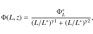
where
After attempting different model fits (i.e., pure luminosity evolution (PLE), pure density evolution (PDE), or a combination
of luminosity and density evolution),
we assumed a luminosity-dependent density evolution model (LDDE) with the parameterization introduced by
Ueda et al. (2003).
From X-ray studies, it is now well established that a LDDE model provides a
more accurate description of the evolutionary properties of AGN (La Franca et al. 2005; Ebrero et al. 2009; Hasinger et al. 2005; Ueda et al. 2003; Silverman et al. 2008), and this is the case also in the optical domain
for at least type-1 AGN (Bongiorno et al. 2007, hereafter B07).
We can describe the LF as a function of redshift with
| (7) |
where
![\begin{displaymath}{\rm e}(z,L) = \left\{
\begin{array}{ll}
(1+z)^{p1} & (z \...
...1+z_{\rm c})]^{p2} & (z > z_{\rm c})\\
\end{array} \right. ,
\end{displaymath}](/articles/aa/full_html/2010/02/aa13229-09/img106.png)
along with
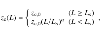
where
Given the small redshift range covered by the data, we are unable to fully constrain the evolution.
For this reason, we fixed the evolutionary parameters (p1, p2, ![]() ,
,
![]() ,
La)
and used the
,
La)
and used the ![]() minimization method to derive the normalization
minimization method to derive the normalization ![]() ,
the characteristic luminosity L*, and the bright and faint end slopes of the LF (
,
the characteristic luminosity L*, and the bright and faint end slopes of the LF (![]() and
and ![]() ).
).
![\begin{figure}
\par\includegraphics[height=12cm,width=12cm,clip]{13229fig11.ps} \end{figure}](/articles/aa/full_html/2010/02/aa13229-09/img111.png)
|
Figure 11: Upper panels: binned [O III] LF of type-2 AGN (black circles for zCOSMOS and blue diamonds for SDSS) and type-1 AGN (orange squares; R08); open symbols show incomplete bins not used to derive the model fit. The curves represent the LF model fit: black for the type-2 AGN model as derived in Sect. 7.1; while orange for the VVDS type-1 AGN sample (B07) appropriately converted from broad-band luminosity to [O III] (see text). Lower panels: fraction of type-2 AGN to the total type-1 + type-2 AGN population. Data points (black circles for zCOSMOS and blue diamonds for SDSS) are derived using the LF data points, while the black line is the resulting fraction considering the LF model fit for type-1 and type-2 AGN. As a comparison, in the first redshift bin, the fraction of obscured AGN derived by Simpson (2005) is overplotted with magenta squares. Finally, the dot-dashed green line is the linear fit to the type-2 fraction found by Hasinger (2008) and converted using the Netzer et al. (2006) relation. |
| Open with DEXTER | |
The evolution parameters were fixed using the results obtained by DC08, appropriately
converted to [O III] luminosity and our cosmology.
By fixing p1=6.5, p2=-1.15,
![]() erg s-1,
erg s-1,
![]() and
and
![]() ,
we obtained
the best-fit model parameters
,
we obtained
the best-fit model parameters
![]() ,
,
![]() ,
and
,
and
![]() erg s-1 with the normalization
erg s-1 with the normalization
![]() Mpc
Mpc![]() .
.
The representation of this best-fit model is shown as a solid line in Fig. 10, where all the data used in the derivation of the model are shown as filled symbols. The dashed line in each panel represents the best-fit model at z=0.
This model represents reasonably well the data points reproducing
the shape of the LF in the first two redshift bins, with a slight underestimation of the bright-end SDSS data points.
The last bin is
not well fitted. In this redshift bin, the LF data points
show an excess in the bright part of the LF. A possible bias could in principle be due to
a higher mean redshift of
the bright objects with respect to the central redshift of the bin due to the increasing space
density of AGN with redshift. However, we tend to exclude this possibility because the four objects
in the most deviant data point at the bright end of the LF have a mean redshift of
![]() and are hence very close to the central redshift of the bin. Upcoming
larger samples (e.g., the 20 k zCOSMOS sample) will provide
superior data statistics and hence an improved constraining power.
and are hence very close to the central redshift of the bin. Upcoming
larger samples (e.g., the 20 k zCOSMOS sample) will provide
superior data statistics and hence an improved constraining power.
7.2 Type-2 AGN fraction
One of the most important open issues regarding absorbed AGN is understanding their relevance amongst the AGN population and if there is a dependence of the fraction of absorbed AGN on either luminosity and/or redshift.
We computed the type-2 AGN fraction, i.e., the ratio of type-2 to total
(type-1 + type-2) AGN, using the derived number densities for the type-2 AGN sample.
In the analyzed redshift range (
0.15<z<0.92), direct [O III] LF measurements for type-1 AGN are
available only at 108.3
![]()
![]() (SDSS; R08). The zCOSMOS
type-2 AGN luminosity regime remains thus mostly uncovered by data.
To constrain also this luminosity range, we have converted the optical broad-band
MB LF derived by B07
for type-1 AGN to a [O III] LF.
The B-band LF computed by B07 ranges from
MB= -20 to
MB = -26 thus probing
the [O III] luminosity interval from
(SDSS; R08). The zCOSMOS
type-2 AGN luminosity regime remains thus mostly uncovered by data.
To constrain also this luminosity range, we have converted the optical broad-band
MB LF derived by B07
for type-1 AGN to a [O III] LF.
The B-band LF computed by B07 ranges from
MB= -20 to
MB = -26 thus probing
the [O III] luminosity interval from ![]() 107.2
107.2 ![]() to
to
![]() 109.5
109.5 ![]() (see Eq. (10)).
(see Eq. (10)).
To do this, following the same approach used by R08, we used the mean
![]() -MB relation
and its scatter
-MB relation
and its scatter ![]() .
The [O III] luminosity is not a perfect tracer of bolometric luminosity and there is indeed
substantial scatter between [O III] and continuum luminosity for type 1
quasars (Netzer et al. 2006, R08).
We thus considered the scatter
.
The [O III] luminosity is not a perfect tracer of bolometric luminosity and there is indeed
substantial scatter between [O III] and continuum luminosity for type 1
quasars (Netzer et al. 2006, R08).
We thus considered the scatter ![]() around the mean
around the mean
![]() -MB relation and
convolved this with the broad-band LF. We assumed a relation between
-MB relation and
convolved this with the broad-band LF. We assumed a relation between
![]() and MB derived for the SDSS type-1 sample by R08 and
converted from a rest-frame wavelength of 2500 Å to the
B-band by adding 0.2
and MB derived for the SDSS type-1 sample by R08 and
converted from a rest-frame wavelength of 2500 Å to the
B-band by adding 0.2![]() , thus obtaining
, thus obtaining
![\begin{displaymath}\log\left(\frac{L_{\rm {[O~{III}]}}}{L_{\odot}}\right)= -0.38~M_{B}-0.42
\end{displaymath}](/articles/aa/full_html/2010/02/aa13229-09/img121.png)
with a scatter in
By convolving the broad-band
LF with the mean
![]() -MB relation with its log-normal scatter (see
Eq. (12) of R08),
we obtain the [O III] LF model for type-1 AGN, which is shown as an orange line in
the three upper panels of Fig. 11, where additionally the SDSS type-1 AGN
[O III] LF data points (derived directly from [O III] luminosities; R08)
are shown as orange squares.
-MB relation with its log-normal scatter (see
Eq. (12) of R08),
we obtain the [O III] LF model for type-1 AGN, which is shown as an orange line in
the three upper panels of Fig. 11, where additionally the SDSS type-1 AGN
[O III] LF data points (derived directly from [O III] luminosities; R08)
are shown as orange squares.
By comparing this to the [O III] LF model derived in the previous section for type-2 AGN (black line in the same panels), we can directly estimate the type-2 AGN fraction in the three redshift bins. This is shown as a solid black line in the lower panels of Fig. 11. We also computed the same quantity by considering the data points instead of the models. In particular, for the type-2 AGN we used the LF data points, while for the type-1 AGN the only data available are from the SDSS (orange squares), and thus in the zCOSMOS regime we continued to use the extrapolated model. The result of this second way of computing the type-2 AGN fraction, is shown with black circles (zCOSMOS) and blue diamonds (SDSS) in the lower panels of Fig. 11. As expected, the two methods are in good agreement and consistent within the errors, which are however, very large.
For the
0.15<z<0.3 bin, we find that the type-2 fraction decreases with
luminosity from ![]() 65% (zCOSMOS data)
to
65% (zCOSMOS data)
to ![]() 50% (SDSS data) going from
50% (SDSS data) going from
![]()
![]() to brighter
luminosities (
to brighter
luminosities (
![]() -109.2
-109.2 ![]() ). However, considering the errors and
taking into account that the fractions derived from SDSS have to be considered as lower limits (see R08),
the trend is also consistent with being constant with luminosity.
At higher redshift, the trend with luminosities is stronger, clearly showing a decreasing fraction of
type-2 AGN with luminosity.
At
0.3<z<0.45 and
0.5<z<0.92, the type-2 fraction ranges from
). However, considering the errors and
taking into account that the fractions derived from SDSS have to be considered as lower limits (see R08),
the trend is also consistent with being constant with luminosity.
At higher redshift, the trend with luminosities is stronger, clearly showing a decreasing fraction of
type-2 AGN with luminosity.
At
0.3<z<0.45 and
0.5<z<0.92, the type-2 fraction ranges from ![]() 80% at
80% at
![]() -108.5
-108.5 ![]() to
to ![]() 25% in the SDSS regime
(
25% in the SDSS regime
(
![]() -109.6
-109.6 ![]() ).
In contrast, we do not detect any clear trend with redshift. At fixed luminosity, e.g.,
).
In contrast, we do not detect any clear trend with redshift. At fixed luminosity, e.g.,
![]()
![]() ,
the fraction slightly increases from 73% to 81% from
,
the fraction slightly increases from 73% to 81% from ![]() to
to ![]() .
However, within the margins of error this is consistent with being constant.
.
However, within the margins of error this is consistent with being constant.
We note that these results are based on two samples (zCOSMOS and SDSS) and that the different selection methods may affect the observed trend. From the COSMOS data points alone, the type-2 fraction appears to be quite constant with luminosity in each redshift bin, although in a more limited luminosity range.
There has been a substantial amount of work to determine the obscured AGN fraction as a function of luminosity and redshift, leading sometimes to contradictory results. In the optical band, Simpson (2005), using a sample of type-1 AGN [O III] selected from the SDSS sample at 0.02<z<0.3, measured a decline in the type-2 fraction with luminosity. His fractions (represented by magenta squares in the first redshift bin) are broadly consistent with our (more uncertain) fractions. In the X-ray band, where most of the work on this topic has been completed, several studies suggest that the fraction of obscured AGN decreases with luminosity and increases with z (La Franca et al. 2005; Ueda et al. 2003; Barger et al. 2005; Sazonov et al. 2007; Treister et al. 2006; Hasinger 2008), while other studies suggest that it is independent of both L and z (Dwelly & Page 2006), or that it is independent of z but not of L (Gilli et al. 2007; Ueda et al. 2003; Akylas et al. 2006).
The comparison of an optical type-2/(type-1 + type-2) fraction with an X-ray obscured/(unobs+obs)
fraction is always affected by limitations and differences related to the AGN classification in
different bands. For example, Compton thick AGN may be missed by X-ray surveys (La Massa et al. 2009),
while the optical selection can fail to select
AGN light diluted by their host galaxy.
Moreover, the redshift range covered by X-ray samples usually extends to higher redshift
than the optical ones.
To overcome the difficulties in classifying either the
optical or the X-ray bands, Hasinger (2008) selected in the 2-10 keV band
a sample of 1290 obscured AGN by combining both diagnostics.
From this sample, he found a significant increase in the absorbed fraction with redshift and confirmed
with higher quality statistics that there is a strong decline
in the same fraction with X-ray luminosities. This decline can be described by an almost
linear decrease from 80% to 20% in the luminosity range
![]() -1046.
We show this trend with a dot-dashed green line in Fig. 11 after converting the X-ray
to [O III] luminosity using the Netzer et al. (2006) relation.
-1046.
We show this trend with a dot-dashed green line in Fig. 11 after converting the X-ray
to [O III] luminosity using the Netzer et al. (2006) relation.
8 Summary and conclusions
We have presented the faintest optically selected sample of type-2 AGN to date.
The sample, selected from the zCOSMOS survey, consists of 213 sources in the redshift
range
0.15<z<0.92, spanning the [O III] luminosity range
![]() .
The only other sample at z>0.15 is one
selected in a similar way from the SDSS by Zakamska et al. (2003), which,
however, covers significantly brighter luminosities (
.
The only other sample at z>0.15 is one
selected in a similar way from the SDSS by Zakamska et al. (2003), which,
however, covers significantly brighter luminosities (
![]() ).
).
Our sample has been selected using the first 10 000 spectra of the zCOSMOS dataset
on the basis of their emission line properties.
In particular, we used the standard BPT diagrams ([O III]/H![]() versus [N II]/H
versus [N II]/H![]() and
[O III]/H
and
[O III]/H![]() versus [S II]/H
versus [S II]/H![]() )
to isolate AGN in the redshift range
0.15<z<0.45 and the
more recent diagnostic diagram [O III]/H
)
to isolate AGN in the redshift range
0.15<z<0.45 and the
more recent diagnostic diagram [O III]/H![]() versus [O II]/H
versus [O II]/H![]() to extend the selection to
higher redshift (
0.5<z<0.92), after applying a cut to the S/N ratio of the involved
lines.
to extend the selection to
higher redshift (
0.5<z<0.92), after applying a cut to the S/N ratio of the involved
lines.
Cross-checking the zCOSMOS emission-line sample with the XMM-COSMOS catalog,
we found a significant incompleteness in the [O II]/H![]() diagnostic
diagram used to select high redshift type-2 AGN (z>0.5).
Our hypothesis is that LINERs
as well as composite AGN/SF sources can be misclassified by this diagram.
diagnostic
diagram used to select high redshift type-2 AGN (z>0.5).
Our hypothesis is that LINERs
as well as composite AGN/SF sources can be misclassified by this diagram.
For the selected type-2 AGN sample, we computed the [O III]![]() 5007
5007![]() line luminosity function using
the
line luminosity function using
the
![]() method.
The selection function takes into account (and corrects for) the sources that were not
spectroscopically observed (but were in the photometric catalog) and those for
which a secure spectroscopic identification has not been obtained. The correction is
performed using a statistical weight associated with each galaxy that has a secure redshift
measurement.
Since the sample was selected from a magnitude-limited sample,
applying a criterion based on the line fluxes, the maximum volume
method.
The selection function takes into account (and corrects for) the sources that were not
spectroscopically observed (but were in the photometric catalog) and those for
which a secure spectroscopic identification has not been obtained. The correction is
performed using a statistical weight associated with each galaxy that has a secure redshift
measurement.
Since the sample was selected from a magnitude-limited sample,
applying a criterion based on the line fluxes, the maximum volume
![]() for
each object has been estimated as the minimum between the volume
for
each object has been estimated as the minimum between the volume
![]() associated with the maximum apparent magnitude and
the volumes
associated with the maximum apparent magnitude and
the volumes
![]() associated with the minimum flux of the used lines.
We have extended the [O III]
associated with the minimum flux of the used lines.
We have extended the [O III]![]() 5007
5007![]() LF to luminosities about 2 orders of magnitude fainter than those previously
available (down to
LF to luminosities about 2 orders of magnitude fainter than those previously
available (down to
![]() ).
).
To enlarge the luminosity range, we combined our faint zCOSMOS sample with the
sample of bright type-2 AGN from the SDSS (R08) and
found that the evolutionary model that represents the combined
luminosity functions most accurately is an LDDE model.
By fixing the evolutionary parameters (p1, p2, ![]() ,
,
![]() ,
La)
using the results obtained by DC08, we obtained
as best-fit model parameters
,
La)
using the results obtained by DC08, we obtained
as best-fit model parameters
![]() ,
,
![]() ,
and
,
and
![]() erg s-1 with the normalization
erg s-1 with the normalization
![]() Mpc-3.
Mpc-3.
Finally, by comparing the LF for type-2 and type-1 AGN (obtained by
converting the broad-band LF from the VVDS into an [O III] LF), we constrained the type-2 quasar fraction as a function
of luminosity. We found that the fraction of type-2 AGN is high at low [O III] luminosities
and then decreases at higher luminosities, in agreement with that found from
several studies in the X-ray band (Gilli et al. 2007; Ueda et al. 2003; Barger et al. 2005; Sazonov et al. 2007; Treister et al. 2006).
The same decreasing trend with luminosity is found in all individual redshift bins,
and we found on average a slightly higher fraction
towards higher redshift
(consistent however with being constant inside the errors).
In particular, we found that at
0.15<z<0.3 the fraction of type-2 AGN decreases with
luminosity from ![]() 65%
to
65%
to ![]() 50%,
while at
0.3<z<0.45, and
0.5<z<0.92 the type-2 fraction ranges from
50%,
while at
0.3<z<0.45, and
0.5<z<0.92 the type-2 fraction ranges from ![]() 80%
to
80%
to ![]() 25%.
However, analysis of a sample uniformly selected across a wider luminosity range is needed to
confirm these results, which are derived by combining two different samples (zCOSMOS and SDSS).
We can not exclude that the observed trend could still be an artifact produced by the different
selection functions in the two samples. From the COSMOS data points alone,
the type-2 fraction seems to be quite constant with luminosity.
25%.
However, analysis of a sample uniformly selected across a wider luminosity range is needed to
confirm these results, which are derived by combining two different samples (zCOSMOS and SDSS).
We can not exclude that the observed trend could still be an artifact produced by the different
selection functions in the two samples. From the COSMOS data points alone,
the type-2 fraction seems to be quite constant with luminosity.
A.B. wishes to thank the referee for the useful suggestions that significantly improved the manuscript. A.B. also thank H. Netzer for the the stimulating discussion, R. Fassbender for helping to improve the manuscript and S. Savaglio for sharing the expertise. This work is based on the zCOSMOS ESO Large Program Number 175.A-0839 and was supported by an INAF contract PRIN/2007/1.06.10.08, and an ASI grant ASI/COFIS/WP3110 I/026/07/0, Partial support of this work is provided by NASA ADP NNX07AT02G, CONACyT 83564, and PAPIITIN110209. These results are also based in part on observations obtained with XMM-Newton, an ESA Science Mission with instruments and contributions directly funded by ESA Member States and the USA (NASA).
References
- Akylas, A., Georgantopoulos, I., Georgakakis, A., Kitsionas, S., & Hatziminaoglou, E. 2006, A&A, 459, 693 [NASA ADS] [CrossRef] [EDP Sciences] [Google Scholar]
- Antonucci, R. 1993, ARA&A, 31, 473 [Google Scholar]
- Baldwin, J. A., Phillips, M. M., & Terlevich, R. 1981, PASP, 93, 5 [NASA ADS] [CrossRef] [EDP Sciences] [Google Scholar]
- Barger, A. J., Cowie, L. L., Mushotzky, R. F., et al. 2005, AJ, 129, 578 [NASA ADS] [CrossRef] [Google Scholar]
- Barth, A. J., Ho, L. C., Filippenko, A. V., & Sargent, W. L. W. 1998, ApJ, 496, 133 [NASA ADS] [CrossRef] [Google Scholar]
- Bennert, N., Falcke, H., Schulz, H., Wilson, A. S., & Wills, B. J. 2002, ApJ, 574, L105 [NASA ADS] [CrossRef] [Google Scholar]
- Bolzonella, M., Kovac, K., Pozzetti, L., et al. 2009 [arXiv:0907.0013] [Google Scholar]
- Bongiorno, A., Zamorani, G., Gavignaud, I., et al. 2007, A&A, 472, 443 [NASA ADS] [CrossRef] [EDP Sciences] [Google Scholar]
- Boyle, B. J., Shanks, T., & Peterson, B. A. 1988, MNRAS, 235, 935 [NASA ADS] [Google Scholar]
- Boyle, B. J., Shanks, T., Croom, S. M., et al. 2000, MNRAS, 317, 1014 [NASA ADS] [CrossRef] [Google Scholar]
- Brusa, M., Zamorani, G., Comastri, A., et al. 2007, ApJS, 172, 353 [NASA ADS] [CrossRef] [Google Scholar]
- Calzetti, D., Kinney, A. L., & Storchi-Bergmann, T. 1994, ApJ, 429, 582 [NASA ADS] [CrossRef] [Google Scholar]
- Capak, P., Aussel, H., Ajiki, M., et al. 2007, ApJS, 172, 99 [NASA ADS] [CrossRef] [Google Scholar]
- Cappelluti, N., Brusa, M., Hasinger, G., et al. 2009, A&A, 497, 635 [NASA ADS] [CrossRef] [EDP Sciences] [Google Scholar]
- Croom, S. M., Smith, R. J., Boyle, B. J., et al. 2004, MNRAS, 349, 1397 [NASA ADS] [CrossRef] [Google Scholar]
- Croom, S. M., Richards, G. T., Shanks, T., et al. 2009, MNRAS, 1439 [Google Scholar]
- Della Ceca, R., Caccianiga, A., Severgnini, P., et al. 2008, A&A, 487, 119 [NASA ADS] [CrossRef] [EDP Sciences] [Google Scholar]
- Dessauges-Zavadsky, M., Pindao, M., Maeder, A., & Kunth, D. 2000, A&A, 355, 89 [NASA ADS] [Google Scholar]
- Dwelly, T., & Page, M. J. 2006, MNRAS, 372, 1755 [NASA ADS] [CrossRef] [Google Scholar]
- Ebrero, J., Carrera, F. J., Page, M. J., et al. 2009, A&A, 493, 55 [NASA ADS] [CrossRef] [EDP Sciences] [Google Scholar]
- Elvis, M., Civano, F., Vignali, C., et al. 2009, ApJS, 184, 158 [NASA ADS] [CrossRef] [Google Scholar]
- Falcke, H., Nagar, N. M., Wilson, A. S., & Ulvestad, J. S. 2000, ApJ, 542, 197 [NASA ADS] [CrossRef] [Google Scholar]
- Fan, X., Strauss, M. A., Schneider, D. P., et al. 2001, AJ, 121, 54 [NASA ADS] [CrossRef] [Google Scholar]
- Fumana, M., Garilli, B., Franzetti, P., et al. 2008, in Astronomical Data Analysis Software and Systems XVII, ed. R. W. Argyle, P. S. Bunclark, & J. R. Lewis, ASP Conf. Ser., 394, 239 [Google Scholar]
- Gilli, R., Comastri, A., & Hasinger, G. 2007, A&A, 463, 79 [NASA ADS] [CrossRef] [EDP Sciences] [Google Scholar]
- González-Martín, O., Masegosa, J., Márquez, I., Guerrero, M. A., & Dultzin-Hacyan, D. 2006, A&A, 460, 45 [NASA ADS] [CrossRef] [EDP Sciences] [Google Scholar]
- Hao, L., Strauss, M. A., Fan, X., et al. 2005a, AJ, 129, 1795 [NASA ADS] [CrossRef] [Google Scholar]
- Hao, L., Strauss, M. A., Tremonti, C. A., et al. 2005b, AJ, 129, 1783 [NASA ADS] [CrossRef] [Google Scholar]
- Hasinger, G. 2008, A&A, 490, 905 [NASA ADS] [CrossRef] [EDP Sciences] [Google Scholar]
- Hasinger, G., Miyaji, T., & Schmidt, M. 2005, A&A, 441, 417 [NASA ADS] [CrossRef] [EDP Sciences] [Google Scholar]
- Hasinger, G., Cappelluti, N., Brunner, H., et al. 2007, ApJS, 172, 29 [NASA ADS] [CrossRef] [Google Scholar]
- Heckman, T. M. 1980, A&A, 87, 142 [NASA ADS] [Google Scholar]
- Heckman, T. M., Ptak, A., Hornschemeier, A., & Kauffmann, G. 2005, ApJ, 634, 161 [NASA ADS] [CrossRef] [Google Scholar]
- Hewett, P. C., Foltz, C. B., Chaffee, F. H., et al. 1991, AJ, 101, 1121 [NASA ADS] [CrossRef] [Google Scholar]
- Ho, L. C. 1999, Adv. Space Res., 23, 813 [NASA ADS] [CrossRef] [Google Scholar]
- Ho, L. C., Filippenko, A. V., & Sargent, W. L. W. 1997, ApJS, 112, 315 [NASA ADS] [CrossRef] [Google Scholar]
- Ho, L. C., Feigelson, E. D., Townsley, L. K., et al. 2001, ApJ, 549, L51 [NASA ADS] [CrossRef] [Google Scholar]
- Huchra, J., & Burg, R. 1992, ApJ, 393, 90 [NASA ADS] [CrossRef] [Google Scholar]
- Huchra, J., Davis, M., Latham, D., & Tonry, J. 1983, ApJS, 52, 89 [NASA ADS] [CrossRef] [Google Scholar]
- Hunt, M. P., Steidel, C. C., Adelberger, K. L., & Shapley, A. E. 2004, ApJ, 605, 625 [NASA ADS] [CrossRef] [Google Scholar]
- Kauffmann, G., Heckman, T. M., Tremonti, C., et al. 2003, MNRAS, 346, 1055 [Google Scholar]
- Kennefick, J. D., Djorgovski, S. G., & de Carvalho, R. R. 1995, AJ, 110, 2553 [NASA ADS] [CrossRef] [Google Scholar]
- Kewley, L. J., Dopita, M. A., Sutherland, R. S., Heisler, C. A., & Trevena, J. 2001, ApJ, 556, 121 [Google Scholar]
- Kewley, L. J., Groves, B., Kauffmann, G., & Heckman, T. 2006, MNRAS, 372, 961 [NASA ADS] [CrossRef] [Google Scholar]
- Koekemoer, A. M., Aussel, H., Calzetti, D., et al. 2007, ApJS, 172, 196 [NASA ADS] [CrossRef] [Google Scholar]
- La Franca, F., Fiore, F., Comastri, A., et al. 2005, ApJ, 635, 864 [NASA ADS] [CrossRef] [Google Scholar]
- La Massa, S. M., Heckman, T. M., Ptak, A., et al. 2009, ApJ, 705, 568 [NASA ADS] [CrossRef] [Google Scholar]
- Lamareille, F. 2010, A&A, 509, A53 [NASA ADS] [CrossRef] [EDP Sciences] [Google Scholar]
- Lamareille, F., Mouhcine, M., Contini, T., Lewis, I., & Maddox, S. 2004, MNRAS, 350, 396 [NASA ADS] [CrossRef] [Google Scholar]
- Lamareille, F., Brinchmann, J., Contini, T., et al. 2009, A&A, 495, 53 [NASA ADS] [CrossRef] [EDP Sciences] [Google Scholar]
- Lilly, S., & Zcosmos Team 2008, The Messenger, 134, 35 [NASA ADS] [Google Scholar]
- Lilly, S. J., Le Fèvre, O., Renzini, A., et al. 2007, ApJS, 172, 70 [NASA ADS] [CrossRef] [Google Scholar]
- Lilly, S. J., LeBrun, V., Maier, C., et al. 2009, ApJS, 184, 218 [Google Scholar]
- Maoz, D., Nagar, N. M., Falcke, H., & Wilson, A. S. 2005, ApJ, 625, 699 [NASA ADS] [CrossRef] [Google Scholar]
- Marshall, H. L., Tananbaum, H., Avni, Y., & Zamorani, G. 1983, ApJ, 269, 35 [NASA ADS] [CrossRef] [Google Scholar]
- McCracken, H. J., Capak, P., Salvato, M., et al. 2009, ApJ, 708, 202 [Google Scholar]
- Mignoli, M., Zamorani, G., Scodeggio, M., et al. 2009, A&A, 493, 39 [NASA ADS] [CrossRef] [EDP Sciences] [Google Scholar]
- Moran, E. C., Lehnert, M. D., & Helfand, D. J. 1999, ApJ, 526, 649 [NASA ADS] [CrossRef] [Google Scholar]
- Mulchaey, J. S., Koratkar, A., Ward, M. J., et al. 1994, ApJ, 436, 586 [NASA ADS] [CrossRef] [Google Scholar]
- Nagar, N. M., Falcke, H., Wilson, A. S., & Ho, L. C. 2000, ApJ, 542, 186 [NASA ADS] [CrossRef] [Google Scholar]
- Netzer, H., Mainieri, V., Rosati, P., & Trakhtenbrot, B. 2006, A&A, 453, 525 [NASA ADS] [CrossRef] [EDP Sciences] [Google Scholar]
- Pei, Y. C. 1995, ApJ, 438, 623 [NASA ADS] [CrossRef] [Google Scholar]
- Pérez-Montero, E., Hägele, G. F., Contini, T., & Díaz, Á. I. 2007, MNRAS, 381, 125 [NASA ADS] [CrossRef] [Google Scholar]
- Reyes, R., Zakamska, N. L., Strauss, M. A., et al. 2008, AJ, 136, 2373 [NASA ADS] [CrossRef] [Google Scholar]
- Rola, C. S., Terlevich, E., & Terlevich, R. J. 1997, MNRAS, 289, 419 [NASA ADS] [Google Scholar]
- Sandage, A., & Tammann, G. A. 1981, S&T, 62, 476 [NASA ADS] [Google Scholar]
- Sanders, D. B., Salvato, M., Aussel, H., et al. 2007, ApJS, 172, 86 [Google Scholar]
- Sazonov, S., Revnivtsev, M., Krivonos, R., Churazov, E., & Sunyaev, R. 2007, A&A, 462, 57 [NASA ADS] [CrossRef] [EDP Sciences] [Google Scholar]
- Schinnerer, E., Smolcic, V., Carilli, C. L., et al. 2007, ApJS, 172, 46 [NASA ADS] [CrossRef] [Google Scholar]
- Schmidt, M. 1968, ApJ, 151, 393 [NASA ADS] [CrossRef] [Google Scholar]
- Schmidt, M., Schneider, D. P., & Gunn, J. E. 1995, AJ, 110, 68 [NASA ADS] [CrossRef] [Google Scholar]
- Scodeggio, M., Franzetti, P., Garilli, B., et al. 2005, PASP, 117, 1284 [NASA ADS] [CrossRef] [Google Scholar]
- Scoville, N., Aussel, H., Brusa, M., et al. 2007, ApJS, 172, 1 [NASA ADS] [CrossRef] [Google Scholar]
- Silverman, J. D., Green, P. J., Barkhouse, W. A., et al. 2008, ApJ, 679, 118 [NASA ADS] [CrossRef] [Google Scholar]
- Simpson, C. 2005, MNRAS, 360, 565 [NASA ADS] [CrossRef] [Google Scholar]
- Stasinska, G., Cid Fernandes, R., Mateus, A., Sodré, L., & Asari, N. V. 2006, MNRAS, 371, 972 [NASA ADS] [CrossRef] [Google Scholar]
- Treister, E., Urry, C. M., & Lira, P. 2006, in Rev. Mex. Astron. Astrofis. Conf. Ser., 26, 147 [Google Scholar]
- Trouille, L., Barger, A. J., Cowie, L. L., Yang, Y., & Mushotzky, R. F. 2009, ApJ, 703, 2160 [NASA ADS] [CrossRef] [Google Scholar]
- Ueda, Y., Akiyama, M., Ohta, K., & Miyaji, T. 2003, ApJ, 598, 886 [NASA ADS] [CrossRef] [Google Scholar]
- Ulvestad, J. S., & Ho, L. C. 2001, ApJ, 558, 561 [NASA ADS] [CrossRef] [Google Scholar]
- Veilleux, S., & Osterbrock, D. E. 1987, ApJS, 63, 295 [NASA ADS] [CrossRef] [Google Scholar]
- Warren, S. J., Hewett, P. C., & Osmer, P. S. 1994, ApJ, 421, 412 [NASA ADS] [CrossRef] [Google Scholar]
- Wolf, C., Wisotzki, L., Borch, A., et al. 2003, A&A, 408, 499 [NASA ADS] [CrossRef] [EDP Sciences] [Google Scholar]
- Zakamska, N. L., Strauss, M. A., Krolik, J. H., et al. 2003, AJ, 126, 2125 [NASA ADS] [CrossRef] [Google Scholar]
- Zhou, H., Wang, T., Yuan, W., et al. 2006, ApJS, 166, 128 [NASA ADS] [CrossRef] [Google Scholar]
- Zucca, E., Bardelli, S., Bolzonella, M., et al. 2009, A&A, 508, 1217 [NASA ADS] [CrossRef] [EDP Sciences] [Google Scholar]
Footnotes
- ... zCOSMOS
- Based on data obtained with the European Southern Observatory Very Large Telescope, Paranal, Chile, program 175.A-0839.
- ...
- Appendix A is only available in electronic form at the CDS via anonymous ftp to cdsarc.u-strasbg.fr (130.79.128.5) or via http://cdsweb.u-strasbg.fr/cgi-bin/qcat?J/A+A/510/A56
- ... objects
- In the selected type-2 AGN sample, 17 sources were compulsory.
- ... adding 0.2
- Assuming the typical spectrum of type-1 AGN, 0.2 is the average color between the rest-frame wavelength of 2500 Å and 4400 Å (B-band).
All Tables
Table 1: Statistic of type-2 AGN and star-forming galaxies among the analyzed emission-line sample for various diagnostic diagrams.
Table 2:
Binned ![]() ([O III]) luminosity function estimates for
([O III]) luminosity function estimates for
![]() ,
,
![]() ,
and
H0=70 km s-1 Mpc-1.
,
and
H0=70 km s-1 Mpc-1.
All Figures
|
|
Figure 1: Observed EWs of the [O III] emission line versus the signal-to-noise ratio of the same line. Grey points represent the parent sample of galaxies in the redshift range considered, while black triangles correspond to the emission-line sample (see text) obtained after applying our selection criteria (S/N([O III]) > 5 and S/N(oth) > 2.5). The dashed line corresponds to the cut in S/N of the [O III] line. Finally, red circles highlight the type-2 AGN sample selected on the basis of the line ratios. The two bottom panels show the EW distribution of the emission-line sample and of the type-2 AGN sample, respectively. |
| Open with DEXTER | |
| In the text | |
|
|
Figure 2:
Examples of zCOSMOS spectra, smoothed by 5 pixels. Upper panels:
four examples of rest-frame spectra with higher [O III] S/N (
|
| Open with DEXTER | |
| In the text | |
|
|
Figure 3:
[
0.15 <z< 0.45]: a) log ([O III]/H |
| Open with DEXTER | |
| In the text | |
|
|
Figure 4:
[
0.5 <z< 0.92]: log ([O III]/H |
| Open with DEXTER | |
| In the text | |
|
|
Figure 5: Redshift and [O III] luminosity distribution of the zCOSMOS type-2 AGN sample (black) compared to the SDSS sample (red) selected by Zakamska et al. (2003). While the redshift ranges are very similar, the luminosity ranges covered by the two samples are complementary. |
| Open with DEXTER | |
| In the text | |
|
|
Figure 6:
As in Figs. 3a and 4, but now showing the positions of X-ray
detected sources. Open and filled symbols correspond to different X-ray luminosities
(open for
|
| Open with DEXTER | |
| In the text | |
|
|
Figure 7: Composite spectrum of X-ray sources optically classified as star-forming galaxies (red line) compared to the composite obtained with all the sources that are not X-ray emitting in the same strip of the star-forming region (black line) and to the composite obtained from the LINER sample selected at low redshift with the BPT diagrams (green line). The lower panel shows the three spectra normalized in the wavelength range around the [O III] line. The comparison between the red and the black line highlights different emission-line strengths ( upper panel) and a redder continuum of the X-ray emitters ( lower panel), suggesting an older stellar population component as well as possible dust extinction on galactic scales. In contrast, the X-ray emitting SFG show properties very similar to the LINER composite (red and green line) in terms of line intensities and continuum shape. |
| Open with DEXTER | |
| In the text | |
|
|
Figure 8:
Observed EWs of the [O III] emission line
versus the signal-to-noise ratio of the continuum close to the line.
Black triangles correspond to the emission-line sample with measured [O III] S/N>5, while red
circles highlight the type-2 AGN sample.
The lower envelope represents the cut in S/N of the line (
|
| Open with DEXTER | |
| In the text | |
|
|
Figure 9:
Binned [O III] line luminosity function of the zCOSMOS type-2 AGN (black circles) derived in the redshift bins
0.15<z<0.3,
0.3<z<0.45, and
0.45<z<0.92, compared to the SDSS (R08) type-2 (blue diamonds) AGN data.
Pink squares show the [2-10 keV] LF derived for the entire (obscured and unobscured) XMM-COSMOS AGN sample
and converted to [O III] luminosities using the Netzer et al. (2006) relation.
The curves in the figure show LF models derived by other authors.
Dot-dashed and dashed lines show the local (z = 0) LF derived from an optically
selected sample (green dot-dashed line; Hao et al. 2005a)
and from an X-ray selected sample (red dashed line; DC08), respectively.
Moreover, in each panel the LF model from
DC08 evolved to the mean redshift of the bin is reported with a solid red line.
The X-ray LF from DC08 was converted to a [O III] LF
using the mean [O III] to X-ray luminosity ratio
derived by Mulchaey et al. (1994) (
|
| Open with DEXTER | |
| In the text | |
|
|
Figure 10: Binned [O III] line luminosity function of zCOSMOS (black circles) and SDSS (blue diamonds) type-2 AGN samples. Open symbols show incomplete bins (see Sect. 7) which were not used to derive the model fits. The black curve in the figure shows the LF best fit model (LDDE) derived considering the combined zCOSMOS-SDSS data shown here. In each panel, the z=0 model is also reported as reference (dashed line). |
| Open with DEXTER | |
| In the text | |
|
|
Figure 11: Upper panels: binned [O III] LF of type-2 AGN (black circles for zCOSMOS and blue diamonds for SDSS) and type-1 AGN (orange squares; R08); open symbols show incomplete bins not used to derive the model fit. The curves represent the LF model fit: black for the type-2 AGN model as derived in Sect. 7.1; while orange for the VVDS type-1 AGN sample (B07) appropriately converted from broad-band luminosity to [O III] (see text). Lower panels: fraction of type-2 AGN to the total type-1 + type-2 AGN population. Data points (black circles for zCOSMOS and blue diamonds for SDSS) are derived using the LF data points, while the black line is the resulting fraction considering the LF model fit for type-1 and type-2 AGN. As a comparison, in the first redshift bin, the fraction of obscured AGN derived by Simpson (2005) is overplotted with magenta squares. Finally, the dot-dashed green line is the linear fit to the type-2 fraction found by Hasinger (2008) and converted using the Netzer et al. (2006) relation. |
| Open with DEXTER | |
| In the text | |
Copyright ESO 2010
Current usage metrics show cumulative count of Article Views (full-text article views including HTML views, PDF and ePub downloads, according to the available data) and Abstracts Views on Vision4Press platform.
Data correspond to usage on the plateform after 2015. The current usage metrics is available 48-96 hours after online publication and is updated daily on week days.
Initial download of the metrics may take a while.