| Issue |
A&A
Volume 513, April 2010
|
|
|---|---|---|
| Article Number | A37 | |
| Number of page(s) | 40 | |
| Section | Cosmology (including clusters of galaxies) | |
| DOI | https://doi.org/10.1051/0004-6361/200912377 | |
| Published online | 21 April 2010 | |
What is a cool-core cluster? a detailed analysis of the cores
of the X-ray flux-limited HIFLUGCS cluster sample![[*]](/icons/foot_motif.png)
D. S. Hudson1 - R. Mittal1,2 - T. H. Reiprich1 - P. E. J. Nulsen3 - H. Andernach1,4 - C. L. Sarazin5
1 - Argelander-Institut für Astronomie der Universität
Bonn, Auf dem Hügel 71, 53121 Bonn, Germany
2 -
Rochester
Institute of Technology, 84 Lamb Memorial Drive, Rochester, NY
14623, USA
3 -
Harvard-Smithsonian Center for Astrophysics, 60 Garden
Street, Cambridge, MA 02138, USA
4 - on leave of absence from
Departamento de Astronomía, Universidad de Guanajuato, AP 144,
Guanajuato CP 36000, Mexico
5 - Department of Astronomy,
University of Virginia, PO Box 400325, Charlottesville, VA
22904-4325, USA
Received 23 April 2009 / Accepted 20 October 2009
Abstract
We use the largest complete sample of 64 galaxy clusters (HIghest
X-ray FLUx Galaxy Cluster Sample) with available high-quality X-ray
data from Chandra, and apply 16 cool-core diagnostics to them, some
of them new. In order to identify the best parameter for
characterizing cool-core clusters and quantify its relation to other
parameters, we mainly use very high spatial resolution profiles of
central gas density and temperature, and quantities derived from
them. We also correlate optical properties of brightest cluster
galaxies (BCGs) with X-ray properties.
To segregate cool core and non-cool-core clusters, we
find that central cooling time,
![]() ,
is the best
parameter for low redshift clusters with high quality data, and that
cuspiness is the best parameter for high redshift clusters. 72% of
clusters in our sample have a cool core (
,
is the best
parameter for low redshift clusters with high quality data, and that
cuspiness is the best parameter for high redshift clusters. 72% of
clusters in our sample have a cool core (
![]() Gyr) and 44% have strong cool cores (
Gyr) and 44% have strong cool cores (
![]() Gyr). We find strong cool-core clusters
are characterized as having low central entropy and a systematic
central temperature drop. Weak cool-core clusters have enhanced
central entropies and temperature profiles that are flat or decrease
slightly towards the center. Non-cool-core clusters have high
central entropies.
Gyr). We find strong cool-core clusters
are characterized as having low central entropy and a systematic
central temperature drop. Weak cool-core clusters have enhanced
central entropies and temperature profiles that are flat or decrease
slightly towards the center. Non-cool-core clusters have high
central entropies.
For the first time we show quantitatively that the discrepancy in classical and spectroscopic mass deposition rates can not be explained with a recent formation of the cool cores, demonstrating the need for a heating mechanism to explain the cooling flow problem.
We find that strong cool-core clusters have a
distribution of central temperature drops, centered on 0.4
![]() .
However, the radius at which the temperature begins to drop
varies. This lack of a universal inner temperature profile probably
reflects the complex physics in cluster cores not directly related
to the cluster as a whole. Our results suggest that the central
temperature does not correlate with the mass of the BCGs and weakly
correlates with the expected radiative cooling only for strong
cool-core clusters. Since 88% of the clusters in our sample have a
BCG within a projected distance of 50
h71-1 kpc from the
X-ray peak, we argue that it is easier to heat the gas (e.g. with
mergers or non-gravitational processes) than to separate the dense
core from the brightest cluster galaxy.
.
However, the radius at which the temperature begins to drop
varies. This lack of a universal inner temperature profile probably
reflects the complex physics in cluster cores not directly related
to the cluster as a whole. Our results suggest that the central
temperature does not correlate with the mass of the BCGs and weakly
correlates with the expected radiative cooling only for strong
cool-core clusters. Since 88% of the clusters in our sample have a
BCG within a projected distance of 50
h71-1 kpc from the
X-ray peak, we argue that it is easier to heat the gas (e.g. with
mergers or non-gravitational processes) than to separate the dense
core from the brightest cluster galaxy.
Diffuse, Mpc-scale radio emission, believed to be associated with major mergers, has not been unambiguously detected in any of the strong cool-core clusters in our sample. Of the weak cool-core clusters and non-cool-core clusters, most of the clusters (seven out of eight) that have diffuse, Mpc-scale radio emission have a large (>50 h71-1 kpc) projected separation between their BCG and X-ray peak. In contrast, only two of the 56 clusters with a small separation between the BCG and X-ray peak (<50 h71-1 kpc) show large-scale radio emission. Based on this result, we argue that a large projected separation between the BCG and the X-ray peak is a good indicator of a major merger. The properties of weak cool-core clusters as an intermediate class of objects are discussed. Finally we describe individual properties of all 64 clusters in the sample.
Key words: intergalactic medium - galaxies: clusters: general
1 Introduction
Early X-ray observations of galaxy clusters revealed that the intracluster medium (ICM) in the centers of many clusters was so dense that the cooling time of the gas was much shorter than the Hubble time (e.g. Fabian & Nulsen 1977; Mathews & Bregman 1978; Cowie & Binney 1977; Lea et al. 1973). These observations led to the development of the cooling flow (CF) model. In this model the ICM at the centers of clusters with dense cores hydrostatically cools, so that the cool gas is compressed by the weight of the overlying gas. Hot gas from the outer regions of the ICM flows in to replace the compressed gas, generating a CF. Although early X-ray observations seemed to corroborate this model and there was some evidence of expected HThe failure of the classical CF model has changed the nomenclature of
these centrally dense clusters from CF clusters to cool-core (CC)
clusters as suggested by Molendi & Pizzolato (2001). One problem with this
nomenclature is that it is unclear what distinguishes a CC cluster
from a non-CC (NCC) cluster. The name implies that gas in the center
of the cluster is cool, but does that always imply a short cooling
time? In fact authors define CC clusters differently often based on
a central temperature drop (e.g. Burns et al. 2008; Sanderson et al. 2006a), short
central cooling time (e.g. Donahue 2007; Bauer et al. 2005; O'Hara et al. 2006), or
significant classical mass deposition rate (Chen et al. 2007). There also
is a question as to whether there is a distinct difference between NCC
and CC clusters. That is, is there a parameter that unambiguously
distinguishes NCC clusters from CC clusters? This is a nontrivial
question since, when used as cosmological probes, clusters are often
segregated into CC/NCC subsamples. Frequently CC clusters are chosen
for mass determination studies since they are believed to be
dynamically relaxed. On the other hand, it requires a large amount of
energy to quench a CF, which may strongly affect the entire ICM. For
example, O'Hara et al. (2006) found that CC clusters (as defined as having
a central cooling time (CCT) more than 3![]() below
7.1
h70-1/2 Gyr) have more scatter about scaling relations
than NCC clusters. Therefore it becomes important to unambiguously
differentiate between CC and NCC clusters before proceeding with
determining their effects on scaling relations.
below
7.1
h70-1/2 Gyr) have more scatter about scaling relations
than NCC clusters. Therefore it becomes important to unambiguously
differentiate between CC and NCC clusters before proceeding with
determining their effects on scaling relations.
It is worth noting that a discrepancy between mass deposition rates determined spectroscopically and those from images in some clusters does not indicate in itself any breakdown of the simple cooling flow picture, since it may be that these clusters just did not have enough time to deposit the predicted level of mass. Here, we will show for the first time that this recent formation solution to the cooling flow discrepancy is very unlikely, based on statistical arguments.
Recently, Chen et al. (2007) investigated the cores of a sample of 106
galaxy clusters based on the extended HIghest X-ray FLUx Galaxy
Cluster Sample (HIFLUGCS) sample (Reiprich & Böhringer 2002) using ROSAT and ASCA, with their primary goal to study the effect
of CC versus NCC clusters on scaling relations. They defined a CC
cluster as one that has significant classically defined mass
deposition rate (
![]() )
and found 49% of their
sample were CC clusters. Additionally they determined that the
fraction of CC clusters in their sample decreased with increasing
mass. Sanderson et al. (2006a) investigated the cores of a statistically
selected sample of the 20 brightest
)
and found 49% of their
sample were CC clusters. Additionally they determined that the
fraction of CC clusters in their sample decreased with increasing
mass. Sanderson et al. (2006a) investigated the cores of a statistically
selected sample of the 20 brightest![]() HIFLUGCS clusters using Chandra. They find that
nine (
HIFLUGCS clusters using Chandra. They find that
nine (![]() 41%) of their clusters are CC clusters, where they define
CC clusters as having a significant drop in temperature in the central
region. Additionally they find that the slope of the inner
temperature profiles has a bimodal distribution with NCC clusters
having a flat temperature profile and CC clusters having a slope
(
41%) of their clusters are CC clusters, where they define
CC clusters as having a significant drop in temperature in the central
region. Additionally they find that the slope of the inner
temperature profiles has a bimodal distribution with NCC clusters
having a flat temperature profile and CC clusters having a slope
(
![]() )
of 0.4. Burns et al. (2008)
investigated the properties of CC and NCC clusters from a cosmological
simulation which produced both types of clusters. As with
Sanderson et al. (2006a), they define CC clusters based on the central
temperature decrease (by 20% of
)
of 0.4. Burns et al. (2008)
investigated the properties of CC and NCC clusters from a cosmological
simulation which produced both types of clusters. As with
Sanderson et al. (2006a), they define CC clusters based on the central
temperature decrease (by 20% of
![]() in their case). Their
simulations show that an early merger determines whether a cluster is
a CC cluster or not and suggest that CC clusters are not necessarily
more relaxed than NCC clusters.
in their case). Their
simulations show that an early merger determines whether a cluster is
a CC cluster or not and suggest that CC clusters are not necessarily
more relaxed than NCC clusters.
Additionally, studies have begun on samples of distant (high-z)
clusters. The goal of these studies is to determine the physical
evolution of CC clusters and whether the CC fraction changes with
redshift. The major obstacle for these high-z cluster studies is
that the traditional indications of CCs are difficult to measure for
distant clusters. Therefore authors offer proxies, based on studies
of low-z clusters, that can be measured for distant clusters with
limited signal. Vikhlinin et al. (2007) suggested cuspiness as a proxy
for determining whether a distant cluster is a CC cluster or not.
Cuspiness is defined as:
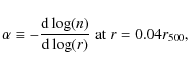
where n is the electron density and r is the distance from the cluster center. For their sample of 20 clusters with z> 0.5, they find a lack of CC clusters. That is, they find no strong CC clusters (
where
In this paper we investigate a statistically complete, flux-limited
sample of 64 X-ray selected clusters and analyze their cores with the
Chandra ACIS instrument. This is the first detailed core
analysis of a nearby, large, complete sample with a high resolution
instrument. With its ![]() 0
0
![]() 5 point spread function, Chandra is the ideal instrument for such a study. Likewise, the
HIFLUGCS sample, which comprises the 64 X-ray brightest clusters
outside the Galactic plane (Reiprich & Böhringer 2002), is an ideal sample.
Since the clusters are bright, they are nearby (
5 point spread function, Chandra is the ideal instrument for such a study. Likewise, the
HIFLUGCS sample, which comprises the 64 X-ray brightest clusters
outside the Galactic plane (Reiprich & Böhringer 2002), is an ideal sample.
Since the clusters are bright, they are nearby (
![]() )
making it possible to probe the very central regions
of the clusters. Moreover they have high signal to noise allowing
precise measurements to be made. It is worth noting that complete
flux-limited samples are not necessarily unbiased or representative
with respect to morphology (e.g. Reiprich 2006). The
point is that, for flux-limited samples, the bias can, in principle,
be calculated (e.g., Ikebe et al. 2002; Stanek et al. 2006). Also,
such samples are representative in the sense that their statistical
properties, like cooling core frequency, are directly comparable to
the same properties of simulated flux-limited samples. Samples
constructed based on availability of data in public archives are, in
general, not representative in this sense (``archive bias'').
)
making it possible to probe the very central regions
of the clusters. Moreover they have high signal to noise allowing
precise measurements to be made. It is worth noting that complete
flux-limited samples are not necessarily unbiased or representative
with respect to morphology (e.g. Reiprich 2006). The
point is that, for flux-limited samples, the bias can, in principle,
be calculated (e.g., Ikebe et al. 2002; Stanek et al. 2006). Also,
such samples are representative in the sense that their statistical
properties, like cooling core frequency, are directly comparable to
the same properties of simulated flux-limited samples. Samples
constructed based on availability of data in public archives are, in
general, not representative in this sense (``archive bias'').
Our goal in this paper is to determine if there is a physical property that can unambiguously segregate CC from NCC clusters. We use this property to examine other parameters to see how well they may be used as proxies when determining whether a cluster is a CC cluster or not. The article is organized as follows. We outline our methods of data reduction in Sect. 2. We present our results in Sect. 3, wherein we describe the various parameters investigated for determining whether a cluster is a CC or an NCC cluster in Sect. 3.1, determine the best parameter to segregate distant CC and NCC clusters in Sect. 3.2, compare this parameter to others in Sect. 3.3 and determine the best diagnostic for cool cores in distant clusters in Sect. 3.4. We discuss our results in Sect. 4, wherein we describe the basic cooling flow problem in Sect. 4.1 and discuss the inner temperature profiles in Sect. 4.2, the central temperature drop seen in some clusters in Sect. 4.2, the relation between cluster mergers and the projected separation between the BCG and X-ray peak in Sect. 4.3 and the WCC clusters in Sect. 4.4. Finally we give our conclusions in Sect. 5. To aid clarity, we give in Table 1 some of the abbreviations used throughout the paper.
Table 1: Nomenclature.
In this work, we assume a flat ![]() CDM Universe with
CDM Universe with
![]() ,
,
![]() ,
and
H0 =
h71 71 km s-1 Mpc-1. Unless otherwise noted, k is
the Boltzmann constant and we use the following nomenclature for our
coordinates: x is the projected distance from the cluster center,
r is the physical 3-D distance from the cluster center and l is
the distance along the line of sight. All errors are quoted at the
1
,
and
H0 =
h71 71 km s-1 Mpc-1. Unless otherwise noted, k is
the Boltzmann constant and we use the following nomenclature for our
coordinates: x is the projected distance from the cluster center,
r is the physical 3-D distance from the cluster center and l is
the distance along the line of sight. All errors are quoted at the
1![]() level unless otherwise noted.
level unless otherwise noted.
2 Observations and methods
All 64 HIFLUGCS clusters have been observed with Chandra,
representing 4.552 Ms of cleaned data. For our analysis we used all
unflared data taken after the CCD focal plane temperature was reduced
to -120![]() C (2001-Jan.-29) and was publicly available as of
2007-May-07, with a few exceptions. (1) In cases where more than one
data set was publicly available and one set was heavily flared, the
entire flared data set was discarded; (2) for A0754
C (2001-Jan.-29) and was publicly available as of
2007-May-07, with a few exceptions. (1) In cases where more than one
data set was publicly available and one set was heavily flared, the
entire flared data set was discarded; (2) for A0754![]() and
A0401
and
A0401![]() ; (3) in the cases of A2597 and A2589 the original
observations were heavily flared and the PIs (Clarke and Buote,
respectively) of the newer proprietary data sets graciously provided
them to us before they became publicly available (4) the Coma Cluster
(A1656), has a recently released calibration observation (2008-Mar.-23)
which we used instead of the pre-2001-Jan.-29 observations. Several
other PI's kindly provided data sets before they were publicly
available, although they since have become publicly available (see
acknowledgments). Details on the number and length of the
observations can be found in Table 2. Note that we use
redshifts compiled from NASA/IPAC Extragalactic Database
(NED)
; (3) in the cases of A2597 and A2589 the original
observations were heavily flared and the PIs (Clarke and Buote,
respectively) of the newer proprietary data sets graciously provided
them to us before they became publicly available (4) the Coma Cluster
(A1656), has a recently released calibration observation (2008-Mar.-23)
which we used instead of the pre-2001-Jan.-29 observations. Several
other PI's kindly provided data sets before they were publicly
available, although they since have become publicly available (see
acknowledgments). Details on the number and length of the
observations can be found in Table 2. Note that we use
redshifts compiled from NASA/IPAC Extragalactic Database
(NED)![]() and the values
did not differ significantly (
and the values
did not differ significantly (
![]() )
from the values used
by Reiprich & Böhringer (2002).
)
from the values used
by Reiprich & Böhringer (2002).
2.1 Data reduction
The basic data reduction was done using CIAO 3.2.2 and CALDB 3.0 following the methods outlined in Hudson et al. (2006). Since we are interested in the cores of clusters, we took the cluster center to be the emission peak (EP) from the background subtracted, exposure corrected image. See Hudson et al. (2006) for details of our image creation technique![\begin{figure}
\par\includegraphics[width=8.5cm,clip]{12377f1.eps}
\end{figure}](/articles/aa/full_html/2010/05/aa12377-09/img55.png)
|
Figure 1: An example of a mosaiced image. This is the background subtracted, exposure corrected image created from the 12 Chandra exposures of A1795. |
| Open with DEXTER | |
2.2 Temperature profiles
Using the EP as the cluster center we created a temperature profile for each cluster using the following method. In order to get good statistics for our temperature profiles, we estimated that 10 000 source counts per annulus would give us a2.3 Cluster virial temperature, radius, and mass
The cluster virial temperature (The temperature decline in the central regions of some clusters, if
included, is the largest source of bias in the determination of
![]() .
The reason for this temperature drop is a current topic
of debate and discussed in more detail in Sect. 4.2. Here
we simply discuss the removal of this central region, so it does not
bias the fit to
.
The reason for this temperature drop is a current topic
of debate and discussed in more detail in Sect. 4.2. Here
we simply discuss the removal of this central region, so it does not
bias the fit to
![]() .
In order to determine the size of the
central region to be excluded, we fit our temperature profiles to a
broken powerlaw. The core radius in the powerlaw was free and
the index of the outer component was fixed to be zero. Additionally we
removed the outer annuli where accurate subtraction of the blank sky
backgrounds (BSB) becomes critical and where clusters may have a
decreasing temperature profile
(De Grandi & Molendi 2002; Vikhlinin et al. 2005; Markevitch et al. 1998;
Burns et al. 2008).
The core radius in the powerlaw was taken to be the radius of the
excluded central region. Table 2 gives this core radius
as well as
.
In order to determine the size of the
central region to be excluded, we fit our temperature profiles to a
broken powerlaw. The core radius in the powerlaw was free and
the index of the outer component was fixed to be zero. Additionally we
removed the outer annuli where accurate subtraction of the blank sky
backgrounds (BSB) becomes critical and where clusters may have a
decreasing temperature profile
(De Grandi & Molendi 2002; Vikhlinin et al. 2005; Markevitch et al. 1998;
Burns et al. 2008).
The core radius in the powerlaw was taken to be the radius of the
excluded central region. Table 2 gives this core radius
as well as
![]() and overall cluster
metalicity. Figure 2 shows examples of the broken powerlaw
fit to the temperature profiles of four representative clusters: (1) a
long exposure of a cluster that has a central temperature drop; (2) a
long exposure of a cluster without a central temperature drop; (3) a
short exposure of a cluster with a central temperature drop and (4) a
short exposure of a cluster without a central temperature drop. If the
core radius in the powerlaw was consistent with zero and/or the
temperature gradient (
and overall cluster
metalicity. Figure 2 shows examples of the broken powerlaw
fit to the temperature profiles of four representative clusters: (1) a
long exposure of a cluster that has a central temperature drop; (2) a
long exposure of a cluster without a central temperature drop; (3) a
short exposure of a cluster with a central temperature drop and (4) a
short exposure of a cluster without a central temperature drop. If the
core radius in the powerlaw was consistent with zero and/or the
temperature gradient (![]() in Col. 5 of Table 3) was
positive, no central region was removed when determining
in Col. 5 of Table 3) was
positive, no central region was removed when determining
![]() .
This method allowed us to take full advantage of the largest
possible signal, while being certain that
.
This method allowed us to take full advantage of the largest
possible signal, while being certain that
![]() was not biased
by cool central gas. Our results suggest that using a fixed fraction
of the virial radius is not efficient and can be dangerous since the
core radius, as defined above, does not scale with the cluster
virial radius.
was not biased
by cool central gas. Our results suggest that using a fixed fraction
of the virial radius is not efficient and can be dangerous since the
core radius, as defined above, does not scale with the cluster
virial radius.
![\begin{figure}
\par\includegraphics[width=8.5cm,clip]{12377f2.eps}
\end{figure}](/articles/aa/full_html/2010/05/aa12377-09/img57.png)
|
Figure 2: These figures show the broken powerlaw fit to four typical temperature profiles representing long and short exposures of clusters with a central temperature drop and clusters without a central temperature drop. The dashed blue lines indicate the fit and the core radius. Top left: A2029 - a long exposure cluster with a central temperature drop. Top right: A3158 - a long exposure of a cluster without a central temperature drop. Bottom left: A3581 - a short exposure of a cluster with a central temperature drop. Bottom right: ZwCl1215 - a short exposure of a cluster without a central temperature drop. |
| Open with DEXTER | |
Since we include all data outside of the core radius when
determining
![]() ,
there are regions where residual background
becomes important. This was especially true for some of our more
distant clusters (e.g. RX J1504,
z = 0.2153). The residual
background results from three factors: (1) since the BSB is scaled to
remove the particle background by matching the BSB 9.5-12 keV rate
to that of the observation, if the scaling factor is much different
from unity, the cosmic X-ray background (CXB) in the BSB will be
significantly increased or decreased before it is subtracted; (2) likewise, the soft CXB component varies over the sky
(e.g. Kuntz 2001) so the CXB in the observation and BSB will be
different and (3) in back-illuminated (BI) CCDs, there are sometimes
residual soft flares. To compensate for these effects a second soft
thermal component was included as well as, in the BI CCDs, an
un-folded powerlaw (i.e. a powerlaw that is not folded through the
instrument response). The temperature of the soft thermal component
was not allowed to exceed 1 keV with a frozen solar abundance and
zero redshift. The normalization of the soft component was also
allowed to be negative in the case of oversubtraction of the CXB
(e.g. for a large scaling factor). For all CCDs of the same type
(i.e. front or back illuminated) in a given observation, we tied the
residual background components with the normalization scaled by area.
We emphasize that for most clusters this step was taken as a
precaution since the cluster emission dominated over the residual CXB.
Only in the most distant clusters of our sample, where the outer
regions are beyond
,
there are regions where residual background
becomes important. This was especially true for some of our more
distant clusters (e.g. RX J1504,
z = 0.2153). The residual
background results from three factors: (1) since the BSB is scaled to
remove the particle background by matching the BSB 9.5-12 keV rate
to that of the observation, if the scaling factor is much different
from unity, the cosmic X-ray background (CXB) in the BSB will be
significantly increased or decreased before it is subtracted; (2) likewise, the soft CXB component varies over the sky
(e.g. Kuntz 2001) so the CXB in the observation and BSB will be
different and (3) in back-illuminated (BI) CCDs, there are sometimes
residual soft flares. To compensate for these effects a second soft
thermal component was included as well as, in the BI CCDs, an
un-folded powerlaw (i.e. a powerlaw that is not folded through the
instrument response). The temperature of the soft thermal component
was not allowed to exceed 1 keV with a frozen solar abundance and
zero redshift. The normalization of the soft component was also
allowed to be negative in the case of oversubtraction of the CXB
(e.g. for a large scaling factor). For all CCDs of the same type
(i.e. front or back illuminated) in a given observation, we tied the
residual background components with the normalization scaled by area.
We emphasize that for most clusters this step was taken as a
precaution since the cluster emission dominated over the residual CXB.
Only in the most distant clusters of our sample, where the outer
regions are beyond ![]() 0.5
0.5
![]() ,
is this correction
essential. As an example the best-fit temperature for RX J1504 without
this correction is 7.1-7.9 keV versus 8.4-10.9 keV with the
residual BSB correction. On the other hand for A0085 (z = 0.055) no
significant difference in temperature is found with or without the
correction.
,
is this correction
essential. As an example the best-fit temperature for RX J1504 without
this correction is 7.1-7.9 keV versus 8.4-10.9 keV with the
residual BSB correction. On the other hand for A0085 (z = 0.055) no
significant difference in temperature is found with or without the
correction.
Once we measured
![]() ,
we used it to determine a
characteristic cluster radius and mass. In the case of radius we used
the scaling relation determined by Evrard et al. (1996):
,
we used it to determine a
characteristic cluster radius and mass. In the case of radius we used
the scaling relation determined by Evrard et al. (1996):
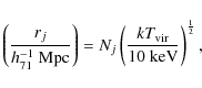
where j is the average overdensity, within rj, above the critical density (
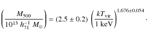
To estimate a characteristic cluster mass (M500), we used the
formulation of Finoguenov et al. (2001) derived from the ROSAT and
ASCA observations of the HIFLUGCS clusters,
2.4 Central temperature drops
To quantify the central temperature drop we calculated two quantities
shown in Cols. 4 and 5 of Table 3. One is simply the
temperature of the central annulus (T0) divided by the virial
temperature (
![]() ). The second is the slope of the powerlaw
fit to the central temperature profile. For clusters with a measured
central temperature drop (Sect. 2.3), we fit the slope out to
the break in the powerlaw. For those clusters with no central
temperature drop, we fit the three innermost annuli
). The second is the slope of the powerlaw
fit to the central temperature profile. For clusters with a measured
central temperature drop (Sect. 2.3), we fit the slope out to
the break in the powerlaw. For those clusters with no central
temperature drop, we fit the three innermost annuli![]() . The purposes of this
measurement was (1) to check for a universal central temperature
profile shape and (2) differentiate between a true systematic drop and
random temperature fluctuations seen in merging clusters (e.g. A0754).
. The purposes of this
measurement was (1) to check for a universal central temperature
profile shape and (2) differentiate between a true systematic drop and
random temperature fluctuations seen in merging clusters (e.g. A0754).
2.5 Density profiles
As with the temperature profile, the surface brightness profile
becomes uncertain at large radii due to uncertainties in the residual
background. Since we are only interested in the central regions and
the surface brightness falls off rapidly at large radii, we focused on
fitting the central regions only. We argue that any uncertainty in
the shape of the profile in the outer regions has a negligible effect
when deprojecting the central regions. Since one of the parameters we
are interested in, cuspiness (see Sect. 2.9 and
Eq. (1)), is defined in terms of the derivative of the
![]() of the density profile at 0.04 r500,
we decided to use a slightly larger (20%) region for determining the
density profiles. This way we would have a constraint on the
derivative of the
of the density profile at 0.04 r500,
we decided to use a slightly larger (20%) region for determining the
density profiles. This way we would have a constraint on the
derivative of the ![]() of the density profile at 0.04 r500.
Specifically, we extracted a spectrum from the projected central
region (0-0.048 r500) and fit it with an absorbed thermal model
(WABS*APEC*EDGE). We used the best-fit parameters of this model to
create a spectrumfile
of the density profile at 0.04 r500.
Specifically, we extracted a spectrum from the projected central
region (0-0.048 r500) and fit it with an absorbed thermal model
(WABS*APEC*EDGE). We used the best-fit parameters of this model to
create a spectrumfile![]() , which we used in turn to
create a weighted exposure map
, which we used in turn to
create a weighted exposure map![]() .
.
We then created a background subtracted, exposure corrected image, in
the 0.5-7.0 keV range, similar to the method described in
Hudson et al. (2006). The difference in our method here and that
described in Hudson et al. (2006) is that: (1) we only used a single
weighted exposure map instead of many monochromatic exposure maps for
different energy bands; (2) we created an error image
(
![]() )
and (3) we created a background subtracted image
with no exposure correction. The error image was created
assuming the errors in the observation, background and readout
artifact or out-of-time events (OOTs) were Poisson (
)
and (3) we created a background subtracted image
with no exposure correction. The error image was created
assuming the errors in the observation, background and readout
artifact or out-of-time events (OOTs) were Poisson (![]()
![]() )
and
could be added in quadrature.
)
and
could be added in quadrature.
We used the background subtracted image with no exposure correction to
determine annuli with at least 500 source counts![]() per annulus and extracted a surface brightness profile and
errors from the background subtracted exposure corrected image and the
error image respectively. The surface brightness profile was then fit
to a single
per annulus and extracted a surface brightness profile and
errors from the background subtracted exposure corrected image and the
error image respectively. The surface brightness profile was then fit
to a single ![]() model:
model:
![\begin{displaymath}\Sigma = \Sigma_{0} \left [ 1 + \left( \frac{x}{x_{\rm c}} \right )^{2} \right ]^{-3\beta + 1/2}
\end{displaymath}](/articles/aa/full_html/2010/05/aa12377-09/img67.png)
or a double
![\begin{displaymath}\Sigma = \Sigma_{01} \left [ 1 + \left( \frac{x}{x_{\rm c_{1}...
...ac{x}{x_{\rm c_{2}}} \right )^{2} \right ]^{-3\beta_{2} + 1/2}
\end{displaymath}](/articles/aa/full_html/2010/05/aa12377-09/img68.png)
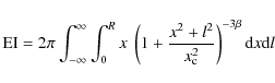
(Cavaliere & Fusco-Femiano 1976), where
From ![]() and
and ![]() for a fit to a
for a fit to a ![]() model (
model (![]() ,
,
![]() ,
,
![]() and
and
![]() for a fit to a double
for a fit to a double ![]() model), we extracted the shape of the density profile.
model), we extracted the shape of the density profile.
![\begin{displaymath}n = n_{0} \left [ 1 + \left ( \frac{r}{r_{\rm c}} \right )^{2} \right ]^{-\frac{3 \beta}{2}}
\end{displaymath}](/articles/aa/full_html/2010/05/aa12377-09/img75.png)
and
![\begin{displaymath}n = \left ( n_{01}^2 \left [ 1 + \left ( \frac{r}{r_{\rm c_1}...
..._2}} \right )^{2} \right ]^{-3 \beta_2} \right )^{\frac{1}{2}}
\end{displaymath}](/articles/aa/full_html/2010/05/aa12377-09/img76.png)
|
(8) |
for a single and double
For a single ![]() model the central electron density, n0 is:
model the central electron density, n0 is:
where
Inserting Eqs. (7) into (10), we get:
for the 0-0.048 r500 region fitted with the APEC model (Mewe et al. 1985; Smith et al. 2001; Mewe et al. 1986; Smith & Brickhouse 2000) and R = 0.048 r500.
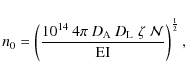
For a double ![]() model the central electron density, n0 is:
model the central electron density, n0 is:
![\begin{displaymath}n_{0} = \left [ \frac{10^{14} \: 4\pi\; (\Sigma_{12}\:{\rm LI...
...EI}_{1} + {\rm LI}_{1}\: {\rm EI}_{2}} \right ]^{\frac{1}{2}},
\end{displaymath}](/articles/aa/full_html/2010/05/aa12377-09/img85.png)
with the same definition of variables as Eq. (9). Additionally,
See Appendix A for details on this calculation.
2.6 Cooling times
Once we created the density profiles, we used them, together with the
cooling function of the best-fit temperature, to estimate the average
cooling time of the gas using:
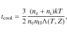
where
where
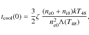
We note here that in order to remove the bias introduced by different
physical resolutions due to different cluster distances, we took any
parameter calculated at r = 0, (e.g. n0 and CCT) to be the
value at
![]() .
The exception to this is
T0, which is defined as the average temperature of the central
annulus, which in all cases had a radius <0.004 r500. We
define
.
The exception to this is
T0, which is defined as the average temperature of the central
annulus, which in all cases had a radius <0.004 r500. We
define
![]() to be the central temperature of the cluster,
either T48 or T0 depending on the parameter considered. In
general
to be the central temperature of the cluster,
either T48 or T0 depending on the parameter considered. In
general
![]() (
(
![]() ).
).
2.7 Entropy
As is typically done in X-ray studies of galaxy clusters, we define entropy as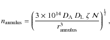
where the variables are defined as before and
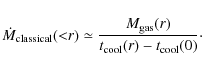
2.8 Mass deposition rates
We define three mass deposition rates: the classically determined mass
deposition rate (
![]() ), the spectrally determined
mass deposition rate (
), the spectrally determined
mass deposition rate (
![]() )
and the modified
spectrally determined mass deposition rate (
)
and the modified
spectrally determined mass deposition rate (
![]() ).
).
![]() is calculated from the gas
density and temperature assuming no energy input. Using the
formulation of Fabian & Nulsen (1979), within radius r,
is calculated from the gas
density and temperature assuming no energy input. Using the
formulation of Fabian & Nulsen (1979), within radius r,
Usually
![]() is a direct measurement of the amount of gas that
is cooling by fitting the expected line emission
(e.g. Peterson et al. 2003) from the multiphase gas. In order to
determine
is a direct measurement of the amount of gas that
is cooling by fitting the expected line emission
(e.g. Peterson et al. 2003) from the multiphase gas. In order to
determine
![]() ,
we fit the 0-0.048 r500 region to
an absorbed thermal model with a cooling flow model
(Mushotzky & Szymkowiak 1988) (WABS*[APEC+MKCFLOW]*EDGE). The higher
temperature component of the cooling flow model was tied to the
thermal model and the lower temperature component was frozen at 0.08 keV.
Given the moderate spectral resolution of the Chandra ACIS, we checked the reliability of the measured values.
Figure 3 shows the comparison between the values obtained
with the XMM RGS and the Chandra ACIS for the nine
clusters in common with our sample and the 14 clusters reported by
Peterson et al. (2003). Figure 3 shows that the values
obtained with the Chandra ACIS are, in all but one
case
,
we fit the 0-0.048 r500 region to
an absorbed thermal model with a cooling flow model
(Mushotzky & Szymkowiak 1988) (WABS*[APEC+MKCFLOW]*EDGE). The higher
temperature component of the cooling flow model was tied to the
thermal model and the lower temperature component was frozen at 0.08 keV.
Given the moderate spectral resolution of the Chandra ACIS, we checked the reliability of the measured values.
Figure 3 shows the comparison between the values obtained
with the XMM RGS and the Chandra ACIS for the nine
clusters in common with our sample and the 14 clusters reported by
Peterson et al. (2003). Figure 3 shows that the values
obtained with the Chandra ACIS are, in all but one
case![]() , consistent with the upper limits obtained by
Peterson et al. (2003). Based on this we argue that the values obtained
with the Chandra ACIS are reliable to well within an order of
magnitude for CC clusters. As we discuss later, this value may not be
accurate for NCC clusters.
, consistent with the upper limits obtained by
Peterson et al. (2003). Based on this we argue that the values obtained
with the Chandra ACIS are reliable to well within an order of
magnitude for CC clusters. As we discuss later, this value may not be
accurate for NCC clusters.
![\begin{figure}
\par\includegraphics[width=7.7cm,clip]{12377f3.eps}
\end{figure}](/articles/aa/full_html/2010/05/aa12377-09/img110.png)
|
Figure 3:
XMM RGS - Chandra ACIS spectroscopic cooling
rates. Here we plot the upper limits measured by Peterson et al. (2003)
with the XMM RGS (black), compared to our Chandra ACIS
measured values (thick red) for the nine clusters in common. For
eight of the nine clusters, the Chandra ACIS gives results
consistent with the XMM RGS. For the one cluster (A2052) for
which they are not consistent, the value measured with the
Chandra ACIS is |
| Open with DEXTER | |
![]() is determined similarly to
is determined similarly to
![]() ,
except that the lower temperature component is left as a free
parameter.
,
except that the lower temperature component is left as a free
parameter.
![]() represents the spectral fit to a
cooling flow model that is stopped at a lower-limit temperature
represents the spectral fit to a
cooling flow model that is stopped at a lower-limit temperature
![]() .
The interpretation of this model is discussed in more
detail in Sect. 4.1.
.
The interpretation of this model is discussed in more
detail in Sect. 4.1.
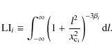
2.9 Cuspiness
Vikhlinin et al. (2007) suggested cuspiness as a proxy for identifying cool-core clusters at large redshift. Equation (1) gives the definition of cuspiness. For our low redshift sample, we can test the correlation of cuspiness with the parameters used to define a cool core. Since our density profile is based on a model, we define it in terms of the model parameters, with r = 0.04 r500. For a single
|
(18) |
For a double
|
(19) |
where
 and
and
 .
.
3 Results
3.1 Bimodality and histograms
In order to determine the best parameter to separate CC clusters from NCC clusters, we tested 16 parameters for bimodality (and trimodality in some cases) using the Kaye's Mixture Model (KMM) algorithm (e.g. Ashman et al. 1994). For each parameter we used a single covariance for both (all three) subgroups when determining the significance of the rejection of the single Gaussian hypothesis. We chose to do this because analytic errors are only statistically meaningful when the same covariance is used for each subgroup. However, since there is no reason to believe the bimodality in any parameter is symmetric, we considered independent covariances for the subgroups when determining the subgroup assignments. Moreover the analytic errors when using different covariances for each subgroup can still give a good guideline on fit improvement (e.g. Ashman et al. 1994), even if their true significance is unknown.
Figure 4 shows histograms of the 16 parameters with Gaussians (created from the KMM algorithm results) overplotted. For each parameter the CC and NCC subgroups were independently determined. We constructed Gaussians using the means and covariances returned by the KMM algorithm and calculated the normalization of the Gaussians so that the integral of the Gaussian was equal to the area of the bins (sum of the number of clusters in each bin times the width of the bin) within its relevant subgroup. Bins of clusters from the CC subgroup are colored blue and bins of clusters from the NCC subgroup are colored red. In the cases with a third subgroup between CC and NCC clusters, the bins are colored black.
![\begin{figure}
\par\includegraphics[width=17cm,clip]{12377f4.eps}
\end{figure}](/articles/aa/full_html/2010/05/aa12377-09/img115.png)
|
Figure 4:
Histograms of 16 parameters that may be used to
distinguish between CC and NCC clusters. Blue bins represent CC
clusters, red bins indicate NCC clusters and where they appear,
black bins represent transitional or weak CC clusters (see
text). Row-wise left to right and starting from the top row the
histograms are: A) central surface brightness (
|
| Open with DEXTER | |
3.1.1 Central surface brightness (A):

The histogram for
3.1.2  model core radius (B):
 (% r500)
In the case of a double 3.1.3 Central electron density (C): n0
The histogram for n0 appears to have a single peak at3.1.4 Central entropy (D): K0
The histogram for K0 looks like it may have a tri-modal
distribution with peaks at ![]() 10
h71-1/3 keV cm2,
10
h71-1/3 keV cm2,
![]() 40
h71-1/3 keV cm2 and
40
h71-1/3 keV cm2 and ![]() 250
h71-1/3 keV cm2. The KMM algorithm rejects the single Gaussian
hypothesis at more than 99% confidence and the likelihood ratio test
statistic (LRTS) (Ashman et al. 1994) suggests K0 is one
of the most significant bimodal distributions. The KMM algorithm
finds a division between the two subgroups at
250
h71-1/3 keV cm2. The KMM algorithm rejects the single Gaussian
hypothesis at more than 99% confidence and the likelihood ratio test
statistic (LRTS) (Ashman et al. 1994) suggests K0 is one
of the most significant bimodal distributions. The KMM algorithm
finds a division between the two subgroups at ![]() 25
h71-1/3 keV cm2, which divides the sample into 27 CC and 37 NCC clusters.
The division in K0 was first reported by Hudson & Reiprich (2007) and
Reiprich & Hudson (2007) and fits well with the results of Voit et al. (2008) and Cavagnolo et al. (2009).
Adding a third subgroup, improves the LRTS further and divides the
distribution at
25
h71-1/3 keV cm2, which divides the sample into 27 CC and 37 NCC clusters.
The division in K0 was first reported by Hudson & Reiprich (2007) and
Reiprich & Hudson (2007) and fits well with the results of Voit et al. (2008) and Cavagnolo et al. (2009).
Adding a third subgroup, improves the LRTS further and divides the
distribution at ![]() 22 and
22 and ![]() 150
h71-1/3 keV cm2,
which gives 24 strong CC (SCC) clusters, 22 weak CC or
transition (WCC) clusters and 18 NCC clusters. The centers of the
subgroups are 11
h71-1/3 keV cm2, 59
h71-1/3 keV cm2 and 257
h71-1/3 keV cm2 for the SCC, WCC and NCC clusters respectively.
150
h71-1/3 keV cm2,
which gives 24 strong CC (SCC) clusters, 22 weak CC or
transition (WCC) clusters and 18 NCC clusters. The centers of the
subgroups are 11
h71-1/3 keV cm2, 59
h71-1/3 keV cm2 and 257
h71-1/3 keV cm2 for the SCC, WCC and NCC clusters respectively.
3.1.5 Biased central entropy (E):

Naïvely one would expect
![]() (see
Eq. (16) for the definition of
(see
Eq. (16) for the definition of
![]() ), however
since
), however
since
![]() is not deprojected and n0 is deprojected,
it is possible that
is not deprojected and n0 is deprojected,
it is possible that
![]() will be larger than n0,
implying an appreciable amount of emission along the line of sight.
This emission increases the apparent central density if it is not
subtracted before determining the central density. In general,
however,
will be larger than n0,
implying an appreciable amount of emission along the line of sight.
This emission increases the apparent central density if it is not
subtracted before determining the central density. In general,
however,
![]() will be smaller than n0, especially
for NCC clusters which require a large region to obtain our count
criterion. The effect of this intentional bias is that NCC clusters
end up with a large value of
will be smaller than n0, especially
for NCC clusters which require a large region to obtain our count
criterion. The effect of this intentional bias is that NCC clusters
end up with a large value of
![]() (as can be seen, the
maximum value of
(as can be seen, the
maximum value of
![]() is larger than the maximum value of
K0). On the other hand CC clusters will have a value of
is larger than the maximum value of
K0). On the other hand CC clusters will have a value of
![]() similar to K0, separating the distribution. The net
effect of the bias seems to be to shift the 15 transition clusters in
the K0 distribution toward the NCC peak. The KMM algorithm
rejects the single Gaussian hypothesis at >99% confidence.
Surprisingly the LRTS suggests the bimodal distribution for
similar to K0, separating the distribution. The net
effect of the bias seems to be to shift the 15 transition clusters in
the K0 distribution toward the NCC peak. The KMM algorithm
rejects the single Gaussian hypothesis at >99% confidence.
Surprisingly the LRTS suggests the bimodal distribution for
![]() is less significant than for K0. The two CC/NCC subgroups are divided at 40
h71-1/3 keV cm2, which gives
29 CC clusters and 35 NCC clusters. The centers of the subgroups are
11
h71-1/3 keV cm2 and 131
h71-1/3 keV cm2 for the CC and NCC clusters respectively.
is less significant than for K0. The two CC/NCC subgroups are divided at 40
h71-1/3 keV cm2, which gives
29 CC clusters and 35 NCC clusters. The centers of the subgroups are
11
h71-1/3 keV cm2 and 131
h71-1/3 keV cm2 for the CC and NCC clusters respectively.
3.1.6 Cooling radius (%
 ) (F)
) (F)
We made two assumptions when calculating the cooling radius:
(1)
![]() (
(
![]() Gyr (see
Sect. 2.8) and (2) the gas at the cooling radius has the density
extrapolated from the 0-0.048 r500 density profile. Therefore,
any cluster with a CCT longer than 7.7
h71-1/2 Gyr, has a
cooling radius of zero. Beyond that, there is a broad distribution
above about
0.02 r500. The KMM algorithm rejects the single
Gaussian hypothesis at 98% confidence, however the algorithm does not
converge if different covariances are used for each subgroup (possibly
because of the large peak at zero). Using a common covariance for the
two subgroups, the KMM algorithm partitions the two subgroups at
0.043 r500 which divides the sample into 37 CC clusters and 27
NCC clusters. The centers of the subgroups are
0.081 r500 and
0.012r500 for the CC and NCC clusters respectively. We note that
since a cluster with
Gyr (see
Sect. 2.8) and (2) the gas at the cooling radius has the density
extrapolated from the 0-0.048 r500 density profile. Therefore,
any cluster with a CCT longer than 7.7
h71-1/2 Gyr, has a
cooling radius of zero. Beyond that, there is a broad distribution
above about
0.02 r500. The KMM algorithm rejects the single
Gaussian hypothesis at 98% confidence, however the algorithm does not
converge if different covariances are used for each subgroup (possibly
because of the large peak at zero). Using a common covariance for the
two subgroups, the KMM algorithm partitions the two subgroups at
0.043 r500 which divides the sample into 37 CC clusters and 27
NCC clusters. The centers of the subgroups are
0.081 r500 and
0.012r500 for the CC and NCC clusters respectively. We note that
since a cluster with
![]() will,
by definition, have cooling radius of zero, it makes a poor parameter
for comparison studies.
will,
by definition, have cooling radius of zero, it makes a poor parameter
for comparison studies.
3.1.7 Scaled spectral mass deposition rate (G):
 /M500
/M500
The histogram for
![]() /M500 shows strong evidence
of a bimodal distribution. There are 13 clusters with a best-fit
value of
/M500 shows strong evidence
of a bimodal distribution. There are 13 clusters with a best-fit
value of
![]() and there is a second peak at
and there is a second peak at
![]() 10-14 h71 yr-1. Since the KMM algorithm was
fitted to the
10-14 h71 yr-1. Since the KMM algorithm was
fitted to the ![]() value of the data, the clusters with
value of the data, the clusters with
![]() ,
were assigned to
,
were assigned to
![]() /(
M500 10-14 h71 yr
-1)] = -5. The KMM
algorithm rejects the single Gaussian hypothesis at >99%
confidence. The LRTS confirms that the bimodality is one of the most
significant of the 16 parameters. The KMM algorithm identifies 23
clusters with the first (NCC) subgroup. However, due to the large
variance in the first subgroup, the two clusters with the largest
value of
/(
M500 10-14 h71 yr
-1)] = -5. The KMM
algorithm rejects the single Gaussian hypothesis at >99%
confidence. The LRTS confirms that the bimodality is one of the most
significant of the 16 parameters. The KMM algorithm identifies 23
clusters with the first (NCC) subgroup. However, due to the large
variance in the first subgroup, the two clusters with the largest
value of
![]() /M500 are assigned to the first
subgroup (see Fig. 4G). Since this is physically
unreasonable, we take the partition value to be
/M500 are assigned to the first
subgroup (see Fig. 4G). Since this is physically
unreasonable, we take the partition value to be ![]()
![]() h71 yr-1, which divides the sample into 43 CC clusters and 21 NCC clusters. The centers of the subgroups are
h71 yr-1, which divides the sample into 43 CC clusters and 21 NCC clusters. The centers of the subgroups are
![]() h71 yr-1 and
h71 yr-1 and
![]() h71 yr-1 for the CC and NCC clusters
respectively. As with cooling radius, the existence of zero values
makes
h71 yr-1 for the CC and NCC clusters
respectively. As with cooling radius, the existence of zero values
makes
![]() /M500 problematic as a parameter for
comparison studies.
/M500 problematic as a parameter for
comparison studies.
3.1.8 Scaled classical mass deposition rate (H):
 /M500
/M500
As with cooling radius, the 18 clusters with CCT >7.7
h71-1/2 Gyr, have
3.1.9 Cuspiness (I): 
The histogram for cuspiness (defined in Eq. (1)) appears
to have a Gaussian distribution around a mean at We note here that for many of the clusters that we have in common with
Vikhlinin et al. (2007), we generally find larger values of ![]() than
they do (based in Fig. 2 in Vikhlinin et al. 2007). There are several
possible explanations for this discrepancy. The most obvious is the
different way in which we calculated r500. We calculated
r500 from
than
they do (based in Fig. 2 in Vikhlinin et al. 2007). There are several
possible explanations for this discrepancy. The most obvious is the
different way in which we calculated r500. We calculated
r500 from
![]() using the formula of Evrard et al. (1996),
which, as we noted earlier, may overestimate r500. On the other
hand Vikhlinin et al. (2007) estimate r500 from their mass model. If
our value of r500 is larger than the value used by
Vikhlinin et al. (2007), it makes sense that our values of
using the formula of Evrard et al. (1996),
which, as we noted earlier, may overestimate r500. On the other
hand Vikhlinin et al. (2007) estimate r500 from their mass model. If
our value of r500 is larger than the value used by
Vikhlinin et al. (2007), it makes sense that our values of ![]() will
be larger, since the profile should steepen around 0.04 r500 (see
Fig. 1 in Vikhlinin et al. 2007). The second major difference is that
our values of
will
be larger, since the profile should steepen around 0.04 r500 (see
Fig. 1 in Vikhlinin et al. 2007). The second major difference is that
our values of ![]() are derived from surface brightness profile
models, whereas Vikhlinin et al. (2007) use direct deprojection and derive
are derived from surface brightness profile
models, whereas Vikhlinin et al. (2007) use direct deprojection and derive
![]() from density profile models. Finally there are minor points
that can contribute to the discrepancies, such as the center used to
create the profile (we both use the X-ray peak, but for some NCC
clusters this is not well-defined), the energy band for the surface
brightness profile and the techniques used to create the profiles. In
the end, we argue that these differences lead to an intrinsic scatter
in the values of
from density profile models. Finally there are minor points
that can contribute to the discrepancies, such as the center used to
create the profile (we both use the X-ray peak, but for some NCC
clusters this is not well-defined), the energy band for the surface
brightness profile and the techniques used to create the profiles. In
the end, we argue that these differences lead to an intrinsic scatter
in the values of ![]() obtained which are dependent on the method
used to determine it.
obtained which are dependent on the method
used to determine it.
3.1.10 Scaled core luminosity (J):
 /[
/[
 ]
]
We define a scaled version of central luminosity ![]() .
Scaled
.
Scaled
![]() is taken from the projected spectral fit to the 0-0.048r500 region. This luminosity is then scaled by
is taken from the projected spectral fit to the 0-0.048r500 region. This luminosity is then scaled by
![]() and the gas mass of the region, calculated from the gas
density profile (
and the gas mass of the region, calculated from the gas
density profile (![]() /[
/[
![]() ]). The
histogram of the scaled
]). The
histogram of the scaled ![]() ,
appears to be a single
distribution with a peak at
,
appears to be a single
distribution with a peak at ![]()
![]() h711/2 erg s-1 keV-1
h711/2 erg s-1 keV-1
![]() .
In fact, the KMM algorithm does not reject the single Gaussian
hypothesis (<40% confidence). If split into a bimodal distribution
the subgroups are partitioned at
.
In fact, the KMM algorithm does not reject the single Gaussian
hypothesis (<40% confidence). If split into a bimodal distribution
the subgroups are partitioned at
![]() h711/2 erg s-1 keV-1
h711/2 erg s-1 keV-1
![]() which divides the sample
into 49 CC clusters and 15 NCC clusters. The centers of the subgroups
are
which divides the sample
into 49 CC clusters and 15 NCC clusters. The centers of the subgroups
are
![]() h711/2 erg s-1 keV-1
h711/2 erg s-1 keV-1
![]() and
and
![]() h711/2 erg s-1 keV-1
h711/2 erg s-1 keV-1
![]() for the CC and NCC clusters
respectively.
for the CC and NCC clusters
respectively.
3.1.11 Central temperature drop (K): T0/

The central temperature drop (T0/
3.1.12 Slope of the inner temperature profile (L)
The histogram for the slopes of the inner temperature profiles does not seem to show any bimodality, suggesting that there is no universal central temperature profile. The fact that T0/3.1.13 Ratio of central temperatures in the soft band to the hard band (M): [T0 (0.5-2.0 keV)]/[T0 (2.0-7.0 keV)]
We also considered fitting the same region to different energy bands in order to identify cool cores. The idea is that if there are many temperatures in the central region the soft band will be more sensitive to the cool gas, whereas the harder band will be more sensitive to the hotter gas. We took our central annulus from the T-profile and fit it in the 0.5-2.0 keV band and then in the 2.0-7.0 keV band and found the ratio. The distribution of values does not look bimodal at all and appears to be a Gaussian centered on3.1.14 Scaled gas mass within 0.048r500 (N):
 /M500
/M500
The high density in the centers of CC clusters suggests that there
should be relatively more gas in the center compared with NCC
clusters. The distribution, however, does not look particularly
bimodal, suggesting that the size of the core does not scale with mass.
There seems to be a peak at 3.1.15 Scaled modified spectral mass deposition rate (O):
 /M500
/M500
The histogram for
3.1.16 Central cooling time (P)
The histogram for CCT looks similar to the histogram of K0, which
is not surprising since they are calculated from similar quantities:
![]()
![]() and n0. Like K0, the histogram of CCT has two
peaks with a smaller peak between the two. The KMM algorithm rejects
the single Gaussian hypothesis at >99% confidence and the LRTS
suggests the bimodality of CCT is the second most significant (after
and n0. Like K0, the histogram of CCT has two
peaks with a smaller peak between the two. The KMM algorithm rejects
the single Gaussian hypothesis at >99% confidence and the LRTS
suggests the bimodality of CCT is the second most significant (after
![]() /M500) among the 16 parameters. As with
K0, adding a third subgroup increases the LRTS. For a bimodal
distribution the partition is
/M500) among the 16 parameters. As with
K0, adding a third subgroup increases the LRTS. For a bimodal
distribution the partition is ![]() 5
h71-1/2 Gyr, which
divides the sample into 42 CC clusters and 22 NCC clusters. For the
tri-modal distribution the CC/NCC partition remains at
5
h71-1/2 Gyr, which
divides the sample into 42 CC clusters and 22 NCC clusters. For the
tri-modal distribution the CC/NCC partition remains at
![]() 5
h71-1/2 Gyr and the SCC/WCC partition is
5
h71-1/2 Gyr and the SCC/WCC partition is
![]() 1
h71-1/2 Gyr. There are four clusters with CCT between
5
h71-1/2 Gyr and 7.7
h71-1/2 Gyr, so that the
difference between a partition at 5
h71-1/2 Gyr and
7.7
h71-1/2 Gyr is a matter of low number statistics. Since
7.7
h71-1/2 Gyr corresponds to a look back time for
1
h71-1/2 Gyr. There are four clusters with CCT between
5
h71-1/2 Gyr and 7.7
h71-1/2 Gyr, so that the
difference between a partition at 5
h71-1/2 Gyr and
7.7
h71-1/2 Gyr is a matter of low number statistics. Since
7.7
h71-1/2 Gyr corresponds to a look back time for ![]() ,
about the time most clusters would have time to relax and form a cool
core, we decided to take the partition as 7.7
h71-1/2 Gyr
rather than 5
h71-1/2 Gyr. Moreover we used
7.7
h71-1/2 Gyr to determine
,
about the time most clusters would have time to relax and form a cool
core, we decided to take the partition as 7.7
h71-1/2 Gyr
rather than 5
h71-1/2 Gyr. Moreover we used
7.7
h71-1/2 Gyr to determine
![]() and
cooling radius. Using 1 and 7.7
h71-1/2 Gyr as cuts we divide
the sample into 28 SCC clusters, 18 WCC clusters and 18 NCC clusters. The centers of the subgroups are 0.45
h71-1/2 Gyr,
1.91
h71-1/2 Gyr and 11.2
h71-1/2 Gyr for the CC, WCC and NCC clusters respectively.
and
cooling radius. Using 1 and 7.7
h71-1/2 Gyr as cuts we divide
the sample into 28 SCC clusters, 18 WCC clusters and 18 NCC clusters. The centers of the subgroups are 0.45
h71-1/2 Gyr,
1.91
h71-1/2 Gyr and 11.2
h71-1/2 Gyr for the CC, WCC and NCC clusters respectively.
Table 4: Summary of the KMM algorithm results for the 16 parameters.
3.2 The defining parameter
The likelihood ratio test identifies
![]() /M500 as having the most significant bimodality,
however we did not choose it as the best method to separate NCC and CC
clusters. There are two reasons for rejecting it as the best method.
(1) Clusters which have a CCT > 7.7
h71-1/2 Gyr have
/M500 as having the most significant bimodality,
however we did not choose it as the best method to separate NCC and CC
clusters. There are two reasons for rejecting it as the best method.
(1) Clusters which have a CCT > 7.7
h71-1/2 Gyr have
![]() ,
making it difficult to compare
,
making it difficult to compare
![]() /M500 to other parameters. (2) The
errors in
/M500 to other parameters. (2) The
errors in
![]() /M500 are quite large (see
Fig. 6G). In fact the average uncertainty in
/M500 are quite large (see
Fig. 6G). In fact the average uncertainty in
![]() /M500 is
/M500 is ![]() 60% versus 15% for CCT,
the parameter with the next most significant bimodality. This
uncertainty is not accounted for in either the histogram or the KMM
algorithm and therefore the significance of the bimodality and the
cluster assignments are also quite uncertain.
60% versus 15% for CCT,
the parameter with the next most significant bimodality. This
uncertainty is not accounted for in either the histogram or the KMM
algorithm and therefore the significance of the bimodality and the
cluster assignments are also quite uncertain.
The parameters with the next highest significance of bimodality are
CCT and K0. As noted earlier, K0 and CCT are both
calculated from n0 and
![]() (in general
(in general
![]() )
and so it is not surprising that they have similar
distributions. Figure 5 shows the tight correlation between
K0 and CCT. The dashed lines show the cut between
CC and WCC clusters for each parameter and the dot-dashed
lines show the cut
between WCC and NCC clusters. There are four clusters which
are
classified as WCC clusters when using K0 and are classified as
SCC clusters when using CCT. It is interesting to note that these
four clusters have the lowest value of K0 for any of the WCC clusters (as classified by K0) and there is also a clear break
(at
)
and so it is not surprising that they have similar
distributions. Figure 5 shows the tight correlation between
K0 and CCT. The dashed lines show the cut between
CC and WCC clusters for each parameter and the dot-dashed
lines show the cut
between WCC and NCC clusters. There are four clusters which
are
classified as WCC clusters when using K0 and are classified as
SCC clusters when using CCT. It is interesting to note that these
four clusters have the lowest value of K0 for any of the WCC clusters (as classified by K0) and there is also a clear break
(at ![]() 30
h71-1/3 keV cm2) between these clusters and
the other WCC clusters (see Fig. 5). As noted earlier this
break has also been reported by Hudson & Reiprich (2007), Reiprich & Hudson (2007),
Voit et al. (2008), and Cavagnolo et al. (2009). Additionally one borderline WCC cluster is
classified as an NCC cluster when using K0 and one borderline NCC cluster is assigned to the WCC subpopulation when classified with
K0. Other than these six borderline cases, all the clusters are
assigned to the same subpopluations whether CCT or K0 is used to
classify them.
30
h71-1/3 keV cm2) between these clusters and
the other WCC clusters (see Fig. 5). As noted earlier this
break has also been reported by Hudson & Reiprich (2007), Reiprich & Hudson (2007),
Voit et al. (2008), and Cavagnolo et al. (2009). Additionally one borderline WCC cluster is
classified as an NCC cluster when using K0 and one borderline NCC cluster is assigned to the WCC subpopulation when classified with
K0. Other than these six borderline cases, all the clusters are
assigned to the same subpopluations whether CCT or K0 is used to
classify them.
![\begin{figure}
\par\includegraphics[width=8.5cm,clip]{12377f5.eps}
\end{figure}](/articles/aa/full_html/2010/05/aa12377-09/img165.png)
|
Figure 5:
This plot shows central
entropy (K0) versus CCT. Since both quantities are derived from
|
| Open with DEXTER | |
Based in Fig. 5, there is not much difference between sorting
the sample using K0 or CCT. Assuming bremsstrahlung emission (i.e.
![]() )
and
)
and
![]() ,
the dependency of the cooling time on the temperature
and density is given by
,
the dependency of the cooling time on the temperature
and density is given by
![]() .
Therefore CCT is more dependent on n than on T, while K0 is
more affected by T. Since the determination of T is more
resolution dependent (i.e. it requires
.
Therefore CCT is more dependent on n than on T, while K0 is
more affected by T. Since the determination of T is more
resolution dependent (i.e. it requires ![]() 100
100![]() more photons
to make a spectrum than one bin in a surface brightness profile), we
argue that
more photons
to make a spectrum than one bin in a surface brightness profile), we
argue that
![]() is a better parameter to use. Furthermore
it is also a more traditional metric and short cooling times are the
physical basis of the cooling flow problem.
is a better parameter to use. Furthermore
it is also a more traditional metric and short cooling times are the
physical basis of the cooling flow problem.
3.2.1 CC fractions in redshift and temperature
We further investigated the subpopulations in the CCT by applying the Wilcoxon rank-sum test (Mann & Whitney 1947; Wilcoxon 1945) to the redshift andTable 5:
Results to the Wilcoxon rank-sum test applied to redshift and
![]() for the CC, SCC, WCC and NCC subpopulations.
for the CC, SCC, WCC and NCC subpopulations.
3.2.2 Bias on CC fractions due to flux-limited nature of the sample
Table 6: Results of simulations done to investigate the impact of selection effects on the observed fractions of SCCs, WCCs, and NCCs.
Flux-limited samples suffer from the well-known Malmquist bias, namely that brighter objects have a higher detection rate than fainter objects. In this section, we address how this bias may affect the observed fractions of SCC, WCC and NCC clusters.
Strong cool-core clusters, owing to their high central densities have
enhanced central X-ray emission. This may result in a higher chance of
their detection and serve as an explanation for observing a higher
fraction of SCC clusters in the
![]() and other flux- or
luminosity-limited samples. Since we have a complete sample, this
calculation can be done. We simulated samples of clusters which follow
the X-ray temperature function given by
and other flux- or
luminosity-limited samples. Since we have a complete sample, this
calculation can be done. We simulated samples of clusters which follow
the X-ray temperature function given by
![]() (Ikebe et al. 2002), in the temperature range (0.001-15) keV
and redshift range 0.00-0.25. From the above it is clear that SCC, WCC
and NCC clusters come from the same parent redshift distribution
within 1-
(Ikebe et al. 2002), in the temperature range (0.001-15) keV
and redshift range 0.00-0.25. From the above it is clear that SCC, WCC
and NCC clusters come from the same parent redshift distribution
within 1-![]() standard deviation. Hence, we assigned to the
clusters random redshifts conforming to the
standard deviation. Hence, we assigned to the
clusters random redshifts conforming to the
![]() law,
where
law,
where ![]() is the luminosity distance. We calculated the
luminosities using three different
is the luminosity distance. We calculated the
luminosities using three different
![]() relations as determined for
each of the three categories, the SCC, WCC, and NCC clusters,
individually (Mittal & Reiprich, in preparation).
relations as determined for
each of the three categories, the SCC, WCC, and NCC clusters,
individually (Mittal & Reiprich, in preparation).
In order to estimate the effect of imposing a flux-limit to a mixed
sample of SCCs, WCCs and NCCs on their resulting fractions, we applied
the
![]() flux-limit,
fx (0.1-2.4) keV
flux-limit,
fx (0.1-2.4) keV
![]() erg s-1 cm-2, to the simulated sample. We tried
two different input sets. In the first (simplest) case, we assumed the
SCCs, WCCs and NCCs to have the same
erg s-1 cm-2, to the simulated sample. We tried
two different input sets. In the first (simplest) case, we assumed the
SCCs, WCCs and NCCs to have the same
![]() slope (3.33). The
normalizations were fixed to those found from the fits to the data. In
the second case, we fixed the slopes for SCCs, WCCs and NCCs to the
fitted values (Mittal & Reiprich, in preparation). We find that
in both the cases the output fractions are indeed biased. In
particular, the output SCC fraction is higher than the input
value. Thus we conclude that in reality the SCCs, WCCs and NCCs may
occur with similar fractions and due to the increased X-ray luminosity
in SCCs, their observed fraction is higher in the present sample.
slope (3.33). The
normalizations were fixed to those found from the fits to the data. In
the second case, we fixed the slopes for SCCs, WCCs and NCCs to the
fitted values (Mittal & Reiprich, in preparation). We find that
in both the cases the output fractions are indeed biased. In
particular, the output SCC fraction is higher than the input
value. Thus we conclude that in reality the SCCs, WCCs and NCCs may
occur with similar fractions and due to the increased X-ray luminosity
in SCCs, their observed fraction is higher in the present sample.
3.3 Cooling time compared to other parameters
In order to study underlying physical relations and correlate simple
observables with those requiring high quality data, we compare 14
parameters![]() from
Fig. 4 to the CCT. The relations are plotted in
Fig. 6. The points are color coded by virial
temperature with the color scale cropped at 10 keV. In order to
quantitatively compare the parameters to CCT, we fit the relations to
powerlaws
from
Fig. 4 to the CCT. The relations are plotted in
Fig. 6. The points are color coded by virial
temperature with the color scale cropped at 10 keV. In order to
quantitatively compare the parameters to CCT, we fit the relations to
powerlaws![]() . Since there were errors on both the parameters
and CCT, we used the bisector linear regression routine, BCES
(Akritas & Bershady 1996), to fit the data. Although some of the
parameters (e.g. K0) had correlated errors with CCT, for simplicity
we assumed them to be independent. Additionally, since the relation
between the CCT and the other parameters seemed to behave differently
for the SCC clusters, we separately fit the SCC clusters and the
non-SCC (WCC and NCC) clusters. The black line gives the best fit for
all clusters, the blue line gives the best-fit line for the SCC
clusters and the red gives best-fit line for the non-SCC clusters.
Table 7 gives the fit values for all 14 parameters
(along with K0) for all three lines.
. Since there were errors on both the parameters
and CCT, we used the bisector linear regression routine, BCES
(Akritas & Bershady 1996), to fit the data. Although some of the
parameters (e.g. K0) had correlated errors with CCT, for simplicity
we assumed them to be independent. Additionally, since the relation
between the CCT and the other parameters seemed to behave differently
for the SCC clusters, we separately fit the SCC clusters and the
non-SCC (WCC and NCC) clusters. The black line gives the best fit for
all clusters, the blue line gives the best-fit line for the SCC
clusters and the red gives best-fit line for the non-SCC clusters.
Table 7 gives the fit values for all 14 parameters
(along with K0) for all three lines.
![\begin{figure}
\par\includegraphics[width=17cm,clip]{12377f6.eps}
\end{figure}](/articles/aa/full_html/2010/05/aa12377-09/img176.png)
|
Figure 6:
A comparison of CCT
with fourteen of the parameters from Fig. 4. Row-wise
left to right and starting from the top row the plots are: A) central surface brightness
|
| Open with DEXTER | |
3.3.1
It has been suggested that the central surface brightness,
![]() ,
is an indicator of CC strength (e.g. O'Hara et al. 2006).
We find a surprising large amount of scatter in the plot of
,
is an indicator of CC strength (e.g. O'Hara et al. 2006).
We find a surprising large amount of scatter in the plot of
![]() versus CCT, especially at short cooling times. Since
n0 is derived from
versus CCT, especially at short cooling times. Since
n0 is derived from
![]() and CCT is derived from n0,
one would naïvely expect a tighter correlation. Since
and CCT is derived from n0,
one would naïvely expect a tighter correlation. Since ![]()
![]() n2 any scatter in the n0 versus CCT relation will be
amplified in the
n2 any scatter in the n0 versus CCT relation will be
amplified in the
![]() versus CCT relation. Not surprisingly,
the outliers at the low end are the lower temperature objects. Since
CCT depends both on n0 and T0, cooler gas will have a
shorter cooling time at the same density. Since cooler clusters are
more likely to be CC clusters than hotter clusters (see
Sect. 3.2), it is not surprising that there is more
scatter for the SCC clusters than for WCC and NCC clusters. When
using
versus CCT relation. Not surprisingly,
the outliers at the low end are the lower temperature objects. Since
CCT depends both on n0 and T0, cooler gas will have a
shorter cooling time at the same density. Since cooler clusters are
more likely to be CC clusters than hotter clusters (see
Sect. 3.2), it is not surprising that there is more
scatter for the SCC clusters than for WCC and NCC clusters. When
using
![]() to identify CC clusters, the scatter will lead to
misidentification; however, adding information about
to identify CC clusters, the scatter will lead to
misidentification; however, adding information about
![]() may
be used to help reduce the scatter.
may
be used to help reduce the scatter.
If
![]() is used to separate the CC and NCC clusters, the WCC
clusters are split into CC and NCC clusters, but not clearly on the
basis of CCT. The WCC clusters with the longest CCTs are classified
as NCC clusters, but the WCC clusters with intermediate CCTs
(
is used to separate the CC and NCC clusters, the WCC
clusters are split into CC and NCC clusters, but not clearly on the
basis of CCT. The WCC clusters with the longest CCTs are classified
as NCC clusters, but the WCC clusters with intermediate CCTs
(![]() 4
h71-1/2 Gyr) and short CCTs
(
4
h71-1/2 Gyr) and short CCTs
(![]() 1-2
h71-1/2 Gyr) are sometimes categorized as CC
clusters and sometimes as NCC clusters. Figure 7 shows
how the correlation becomes tighter if the central surface brightness
is scaled by
1-2
h71-1/2 Gyr) are sometimes categorized as CC
clusters and sometimes as NCC clusters. Figure 7 shows
how the correlation becomes tighter if the central surface brightness
is scaled by
![]() .
Cutting
.
Cutting
![]() /
/
![]() at
at
![]() photons cm-2 s-1 keV-1successfully separates the SCC and NCC clusters, with five
misclassified WCC clusters, all but one (A2634) with relatively long
CCTs (>3
h71-1/2 Gyr).
photons cm-2 s-1 keV-1successfully separates the SCC and NCC clusters, with five
misclassified WCC clusters, all but one (A2634) with relatively long
CCTs (>3
h71-1/2 Gyr).
![\begin{figure}
\par\includegraphics[width=8.5cm,clip]{12377f7.eps}
\end{figure}](/articles/aa/full_html/2010/05/aa12377-09/img180.png)
|
Figure 7:
The scaled central surface brightness
|
| Open with DEXTER | |
3.3.2  )
)
We checked to see if there was any correlation between CCT and ![]() as a percentage of r500. We expected a correlation since CC clusters usually require a double
as a percentage of r500. We expected a correlation since CC clusters usually require a double ![]() model to fit their surface
brightness profile, whereas NCC clusters do not. Therefore we expected
model to fit their surface
brightness profile, whereas NCC clusters do not. Therefore we expected
![]() /r500 to be much smaller for CC clusters than NCC clusters. Surprisingly the correlation appears to be tighter than for
/r500 to be much smaller for CC clusters than NCC clusters. Surprisingly the correlation appears to be tighter than for
![]() ,
although there is still a lot of scatter. The KMM determined cut
would classify four SCC clusters as well as most of the
WCC clusters as NCC clusters. If we put the cut at 0.03 r500(just after the third peak in the histogram counting from the left),
however, we would more successfully separate the CC clusters and NCC
clusters. On the other hand, this parameter does a poor job of
separating SCC and WCC clusters. An interesting note is that the
coolest clusters (groups) appear to have smaller values of
,
although there is still a lot of scatter. The KMM determined cut
would classify four SCC clusters as well as most of the
WCC clusters as NCC clusters. If we put the cut at 0.03 r500(just after the third peak in the histogram counting from the left),
however, we would more successfully separate the CC clusters and NCC
clusters. On the other hand, this parameter does a poor job of
separating SCC and WCC clusters. An interesting note is that the
coolest clusters (groups) appear to have smaller values of
![]() /r500 compared to hotter clusters.
/r500 compared to hotter clusters.
3.3.3 n0
There is a tight correlation between n0 and CCT. This is not
surprising since, as noted earlier, n0 is the strongest factor in
determining CCT. All the SCC clusters are CC clusters when determined
with n0 and, similarly, both methods agree on the NCC clusters as
well. The WCC clusters are split at CCT ![]() 2
h71-1/2 Gyr into nine CC and nine being NCC when determined
by n0. It is impossible to separate SCC and WCC clusters using
n0. This suggests that the difference between SCC and WCC
clusters with similar values of n0 is that SCC clusters have a
lower central temperature. This may be due to the central temperature
drop seen in SCC clusters or simply that these SCC clusters are cooler
than their WCC counterparts. Considering NCC and WCC clusters with
similar values of n0, the WCC clusters must be cooler than their
NCC counterparts.
2
h71-1/2 Gyr into nine CC and nine being NCC when determined
by n0. It is impossible to separate SCC and WCC clusters using
n0. This suggests that the difference between SCC and WCC
clusters with similar values of n0 is that SCC clusters have a
lower central temperature. This may be due to the central temperature
drop seen in SCC clusters or simply that these SCC clusters are cooler
than their WCC counterparts. Considering NCC and WCC clusters with
similar values of n0, the WCC clusters must be cooler than their
NCC counterparts.
3.3.4
As with central entropy,
![]() seems to form a tight
correlation with CCT. The KMM break separates the SCC clusters from
the other clusters (with one exception). Perhaps the most interesting
aspect of
seems to form a tight
correlation with CCT. The KMM break separates the SCC clusters from
the other clusters (with one exception). Perhaps the most interesting
aspect of
![]() is that the slope seems to break between the
CC and NCC clusters. Unlike many of the other parameters this looks
truly like a broken powerlaw, as fits to both the SCC and WCC/NCC
clusters have similar values at the transition between them. This
appears to be a good parameter for determining CC and NCC clusters,
although ideally the redshift and observation length biases would need
to be removed. The merging cluster A3266 is the outlier with
CCT
is that the slope seems to break between the
CC and NCC clusters. Unlike many of the other parameters this looks
truly like a broken powerlaw, as fits to both the SCC and WCC/NCC
clusters have similar values at the transition between them. This
appears to be a good parameter for determining CC and NCC clusters,
although ideally the redshift and observation length biases would need
to be removed. The merging cluster A3266 is the outlier with
CCT ![]() 7.7
h71-1/2 and
7.7
h71-1/2 and
![]() keV cm2.
keV cm2.
3.3.5 Cooling radius (%

Since the cooling radius is defined at
![]() h71-1/2 Gyr, the NCC clusters have no cooling radius by
definition. These clusters were excluded when fitting the relation
between cooling radius and CCT. There seems to be a trend of
increasing cooling radius with decreasing cooling time for the WCC
clusters. The SCC clusters, however, do not seem to have any trend
between cooling time and size of the cooling region (as a fraction of
the virial radius). Therefore we can conclude that the density
gradients for SCC clusters vary greatly. The large outliers are:
S1101 at the high end with a cooling radius of >0.15 r500 and
the Fornax cluster at the low end.
h71-1/2 Gyr, the NCC clusters have no cooling radius by
definition. These clusters were excluded when fitting the relation
between cooling radius and CCT. There seems to be a trend of
increasing cooling radius with decreasing cooling time for the WCC
clusters. The SCC clusters, however, do not seem to have any trend
between cooling time and size of the cooling region (as a fraction of
the virial radius). Therefore we can conclude that the density
gradients for SCC clusters vary greatly. The large outliers are:
S1101 at the high end with a cooling radius of >0.15 r500 and
the Fornax cluster at the low end.
3.3.6 Scaled spectral mass deposition rate
This plot explicitly demonstrates the danger of using
![]() to divide the distribution. The error bars that are not
visible in the histogram and not considered in the KMM-algorithm, show
how much overlap there is within errors. There seems to be only a
very weak trend with CCT, especially if the upper limits are included.
The clusters with the highest values of
to divide the distribution. The error bars that are not
visible in the histogram and not considered in the KMM-algorithm, show
how much overlap there is within errors. There seems to be only a
very weak trend with CCT, especially if the upper limits are included.
The clusters with the highest values of
![]() /M500, however, are SCC clusters. As noted earlier and
discussed in more detail later, several of the NCC clusters have
non-negligible spectral mass deposition rates. This fact along with
the spread in values for the SCC clusters makes it very difficult to
use
/M500, however, are SCC clusters. As noted earlier and
discussed in more detail later, several of the NCC clusters have
non-negligible spectral mass deposition rates. This fact along with
the spread in values for the SCC clusters makes it very difficult to
use
![]() to identify CC and NCC clusters, at least
with the spectral resolution of the Chandra ACIS.
to identify CC and NCC clusters, at least
with the spectral resolution of the Chandra ACIS.
3.3.7 Scaled classical mass deposition rate
As with cooling radius,
![]() is defined as zero
for the NCC clusters (clusters with CCT > 7.7
h71-1/2 Gyr),
so these clusters were omitted when fitting the comparison of
is defined as zero
for the NCC clusters (clusters with CCT > 7.7
h71-1/2 Gyr),
so these clusters were omitted when fitting the comparison of
![]() /M500 to CCT. There appears to be a
weak trend of increasing
/M500 to CCT. There appears to be a
weak trend of increasing
![]() /M500 with
decreasing CCT, albeit with a great deal of scatter. We attribute
this scatter to the differences in the gradients of the density
profiles. That is, clusters with a very steep density gradient will
have a very short CCT but not a large value of
/M500 with
decreasing CCT, albeit with a great deal of scatter. We attribute
this scatter to the differences in the gradients of the density
profiles. That is, clusters with a very steep density gradient will
have a very short CCT but not a large value of
![]() ,
whereas clusters with relatively dense cores but
flatter density gradients will have a longer CCT but a large
,
whereas clusters with relatively dense cores but
flatter density gradients will have a longer CCT but a large
![]() .
Based on the KMM determined cut of
.
Based on the KMM determined cut of
![]() h71-1 yr-1 for
h71-1 yr-1 for
![]() /M500, all the SCC clusters are classified as CC
clusters and all but three of the WCC clusters are classified as CC
clusters. Two of these WCC clusters are borderline cases.
/M500, all the SCC clusters are classified as CC
clusters and all but three of the WCC clusters are classified as CC
clusters. Two of these WCC clusters are borderline cases.
There are six WCC clusters (IIIZw54, A1650, A1651, A2142, A2244 and
A4038) that have
![]() /
/
![]() h71-1 yr-1, more consistent with SCC clusters,
although toward the lower end of the SCC clusters. There are five SCC
clusters (A0262, MKW4, NGC 4636, A3526 and A1644) that have
h71-1 yr-1, more consistent with SCC clusters,
although toward the lower end of the SCC clusters. There are five SCC
clusters (A0262, MKW4, NGC 4636, A3526 and A1644) that have
![]() /
/
![]() h71-1 yr-1, more consistent with WCC clusters.
There are four (one SCC and three WCC clusters) outliers that have
very low values of
h71-1 yr-1, more consistent with WCC clusters.
There are four (one SCC and three WCC clusters) outliers that have
very low values of
![]() /M500 (i.e. <
/M500 (i.e. <
![]() h71-1 yr-1). They are: NGC 1399,
A3266, A3667 and A2634. It is interesting to note that all but two of
the low
h71-1 yr-1). They are: NGC 1399,
A3266, A3667 and A2634. It is interesting to note that all but two of
the low
![]() /M500 SCC clusters are low
temperature (kT < 2.5 keV) systems, in fact they are four of the
nine coolest systems. For the ten coolest systems,
/M500 SCC clusters are low
temperature (kT < 2.5 keV) systems, in fact they are four of the
nine coolest systems. For the ten coolest systems,
![]() /M500 is less than
/M500 is less than
![]() yr-1, which is below the average for the
SCC clusters. The WCC outliers are all merging systems suggesting
current cool-core survival, but with some disruption of the cool core.
yr-1, which is below the average for the
SCC clusters. The WCC outliers are all merging systems suggesting
current cool-core survival, but with some disruption of the cool core.
3.3.8 Cuspiness
Cuspiness shows a lot of scatter when compared to CCT. It seems to do
a good job in identifying NCC clusters; only three NCC clusters have
![]() .
All the SCC clusters have
.
All the SCC clusters have
![]() ,
but not all
of them have
,
but not all
of them have
![]() as suggested by Vikhlinin et al. (2007).
Using the KMM determined cut of
as suggested by Vikhlinin et al. (2007).
Using the KMM determined cut of
![]() ,
several of the SCC and
all of the WCC would be classified as NCC clusters. Likewise, using
the cuts of Vikhlinin et al. (2007), seven of the WCC clusters would be
SCC clusters, three of the SCC clusters would be WCC clusters and four
of the WCC clusters would be classified as NCC clusters. Looking at
the fit to the data, there appears to be a shift in normalization and
slope for the SCC clusters. That is, cuspiness increases with shorter
CCTs. However, below CCT
,
several of the SCC and
all of the WCC would be classified as NCC clusters. Likewise, using
the cuts of Vikhlinin et al. (2007), seven of the WCC clusters would be
SCC clusters, three of the SCC clusters would be WCC clusters and four
of the WCC clusters would be classified as NCC clusters. Looking at
the fit to the data, there appears to be a shift in normalization and
slope for the SCC clusters. That is, cuspiness increases with shorter
CCTs. However, below CCT ![]() 1
h71-1/2, the cuspiness drops
suddenly (or at least there is a large range of values). Below a CCT
of
1
h71-1/2, the cuspiness drops
suddenly (or at least there is a large range of values). Below a CCT
of ![]() 1
h71-1/2 Gyr, the cuspiness increases more rapidly
as the CCTs get shorter.
1
h71-1/2 Gyr, the cuspiness increases more rapidly
as the CCTs get shorter.
3.3.9 Scaled central luminosity
Scaled central luminosity (![]() /[
/[
![]()
![]() ])
shows a rather flat but clear relation with CCT, with large scatter
and larger uncertainties. Using the KMM determined cut, however, only
one SCC cluster is misclassified as an NCC cluster. Some of the WCC
clusters are classified as CC clusters and some as NCC clusters when
using the KMM determined cut in scaled central luminosity. If the cut
is raised to
])
shows a rather flat but clear relation with CCT, with large scatter
and larger uncertainties. Using the KMM determined cut, however, only
one SCC cluster is misclassified as an NCC cluster. Some of the WCC
clusters are classified as CC clusters and some as NCC clusters when
using the KMM determined cut in scaled central luminosity. If the cut
is raised to
![]() h711/2 erg s-1 keV
h711/2 erg s-1 keV
![]() ,
still only one SCC cluster is
misclassified, and the number of misclassified NCC clusters is reduced
to two. Unlike, e.g. n0, there seems to be no trend with the CCT
of the WCC and whether it is classified as CC or NCC when using scaled
central luminosity. As with many parameters the relation seems to get
steeper for the SCC clusters.
,
still only one SCC cluster is
misclassified, and the number of misclassified NCC clusters is reduced
to two. Unlike, e.g. n0, there seems to be no trend with the CCT
of the WCC and whether it is classified as CC or NCC when using scaled
central luminosity. As with many parameters the relation seems to get
steeper for the SCC clusters.
3.3.10 T0/
The most interesting feature in this plot is the break in the
distribution for the SCC clusters. Although there is a lot of scatter,
there is a clear drop in central temperature for SCC clusters.
However, the value of the drop seems to be independent of CCT. There
are a few NCC clusters with central temperature drops, most notably
A2256. This may be due to a recent merger in which a core has not yet
been completely destroyed (although a possible dense core has been
disrupted).
Sanderson et al. (2006a) suggested a similar parameter for dividing CC and
NCC clusters. Their parameter is roughly the inverse of
T0/
![]() (T-ratio
(T-ratio ![]()
![]() /
/
![]() ). The major difference being that
). The major difference being that
![]() is defined
as the temperature within 0.1r500, in general much larger than
the region we used to measure T0. They then define CC
significance, which is the difference (in units of
is defined
as the temperature within 0.1r500, in general much larger than
the region we used to measure T0. They then define CC
significance, which is the difference (in units of ![]() )
between
T-ratio and unity
(i.e.
)
between
T-ratio and unity
(i.e.
![]() ). They define
a CC cluster as any cluster with CC significance >3 (i.e. a
significant drop in temperature). Since they use a bright subsample of
HIFLUGCS, all 20 of their clusters are in our sample. We find
that all their CC clusters are SCC clusters in our sample. Their NCC
clusters are either WCC or NCC clusters. Likewise, employing their
method, using
). They define
a CC cluster as any cluster with CC significance >3 (i.e. a
significant drop in temperature). Since they use a bright subsample of
HIFLUGCS, all 20 of their clusters are in our sample. We find
that all their CC clusters are SCC clusters in our sample. Their NCC
clusters are either WCC or NCC clusters. Likewise, employing their
method, using
![]() /T0, we find good agreement with their
classification. On the other hand we argue the values of CC
significance are very sensitive to the uncertainties in T0 and
/T0, we find good agreement with their
classification. On the other hand we argue the values of CC
significance are very sensitive to the uncertainties in T0 and
![]() .
That is if T-ratio
.
That is if T-ratio ![]() 1, then the longer the
observing time the larger CC significance becomes and the more likely
the cluster will be classified as a CC cluster. However, we concur
with their result that in general SCC clusters have a central
temperature drop and that WCC and NCC clusters have a shallow or no
central temperature drop.
1, then the longer the
observing time the larger CC significance becomes and the more likely
the cluster will be classified as a CC cluster. However, we concur
with their result that in general SCC clusters have a central
temperature drop and that WCC and NCC clusters have a shallow or no
central temperature drop.
3.3.11 Slope of the temperature profile
Like T0/3.3.12 [T0 (0.5-2.0 keV)]/[T0 (2.0-7.0 keV)]
[T0 (0.5-2.0 keV)]/[T0 (2.0-7.0 keV)] appears to be a
very poor parameter for identifying CC clusters. As with
![]() ,
it is possible that multiple temperatures along
the line of sight (e.g. from a merging system) can produce results
that make an NCC cluster appear to be a CC cluster. In fact the best
fit (albeit a very poor fit) shows a positive trend rather than the
expected negative trend. Additionally, an NCC cluster (A1656) shows
the smallest fractional value.
,
it is possible that multiple temperatures along
the line of sight (e.g. from a merging system) can produce results
that make an NCC cluster appear to be a CC cluster. In fact the best
fit (albeit a very poor fit) shows a positive trend rather than the
expected negative trend. Additionally, an NCC cluster (A1656) shows
the smallest fractional value.
3.3.13 /M500
![\begin{figure}
\par\includegraphics[width=8.5cm]{Mg_over_kT_vs_CCT.eps}
\end{figure}](/articles/aa/full_html/2010/05/aa12377-09/img194.png)
|
Figure 8:
This figure shows
that that
|
| Open with DEXTER | |
3.3.14 Scaled modified spectral mass deposition rate
As with
![]() /M500, the large uncertainty in
/M500, the large uncertainty in
![]() /M500 shows the limitations of the
histogram. However,
/M500 shows the limitations of the
histogram. However,
![]() /M500 does show a trend
with cooling time, albeit with a large scatter. The fact that it
shows a trend is interesting since CCT and
/M500 does show a trend
with cooling time, albeit with a large scatter. The fact that it
shows a trend is interesting since CCT and
![]() are
independently determined. See Sect. 4.1 for a further
discussion on
are
independently determined. See Sect. 4.1 for a further
discussion on
![]() .
.
Table 7:
The best-fit parameters for the 15 investigated CCT versus parameter. The parameters were fit to CCT = CCT0 (
![]() .
.
3.4 What is the best diagnostic of CC clusters?
One large problem in studying the evolution of CC cluster fraction is that resolving the cores of clusters is difficult for distant clusters. In Sect. 3.3 we compared various parameters to CCT. Not surprisingly n0 and K0 provide the tightest correlation to CCT. In distant clusters n0 is slightly easier to determine than CCT and K0 since it requires no spectral information from the central region. On the other hand it is still dependent on one being able to resolve the very center of the cluster, so it is not the ideal parameter to determine whether a distant cluster is a CC or NCC cluster.
Unfortunately, when compared to n0 and K0, most of the other
parameters show a lot of scatter in their relation with CCT. Of those
other parameters
![]() appears to show the tightest
correlation. Unlike K0,
appears to show the tightest
correlation. Unlike K0,
![]() is not dependent on
n0, but on the average density in a somewhat larger region. It
is therefore not limited by the need to resolve the central region.
There are, however, two problems with using
is not dependent on
n0, but on the average density in a somewhat larger region. It
is therefore not limited by the need to resolve the central region.
There are, however, two problems with using
![]() as a proxy:
(1) it requires a large enough region to fit a spectrum (which can be
physically quite large for distant clusters) and (2) the size of the
region from which
as a proxy:
(1) it requires a large enough region to fit a spectrum (which can be
physically quite large for distant clusters) and (2) the size of the
region from which
![]() is determined differs between
observations (i.e. it is dependent mainly on observing time and
redshift). As a solution to (1) we suggest that the normalization of
the thermal model is not as difficult to constrain as the temperature
or metalicity (not as many counts are needed). In extreme cases the
temperature and metalicity could be frozen at their overall cluster
values so that only the central normalization would need to be
constrained. As a solution to (2) we suggest that the region size be
defined such that it is only dependent on the density profile and is
independent of redshift, temperature and observing time. Specifically
if two clusters have identical density profiles, then
is determined differs between
observations (i.e. it is dependent mainly on observing time and
redshift). As a solution to (1) we suggest that the normalization of
the thermal model is not as difficult to constrain as the temperature
or metalicity (not as many counts are needed). In extreme cases the
temperature and metalicity could be frozen at their overall cluster
values so that only the central normalization would need to be
constrained. As a solution to (2) we suggest that the region size be
defined such that it is only dependent on the density profile and is
independent of redshift, temperature and observing time. Specifically
if two clusters have identical density profiles, then
![]() should be derived from physical regions of the same size.
should be derived from physical regions of the same size.
We suggest using a constant value of the projected emission measure in
a cylinder,
to determine region sizes that depend only on the density profile. Here we define
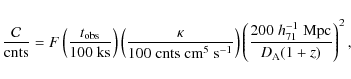
|
(21) |
where
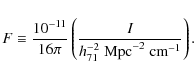
|
(22) |
A value of
Although this method makes the
![]() region size consistent
among clusters, there is an additional problem that a reasonable value
of I at one redshift will often be unreasonable for clusters at a
significantly different redshift. For instance, for our proposed
value of
region size consistent
among clusters, there is an additional problem that a reasonable value
of I at one redshift will often be unreasonable for clusters at a
significantly different redshift. For instance, for our proposed
value of
![]() h71-2 cm-3, which
leads to a 10 000 count region for our median cluster parameters,
would produce a 58 count region for a cluster with identical
parameters but at a redshift of z = 0.5. However, if the region size
is not constant for all studies (say the chosen value of I varies
depending on the study), it makes comparisons between studies
difficult.
h71-2 cm-3, which
leads to a 10 000 count region for our median cluster parameters,
would produce a 58 count region for a cluster with identical
parameters but at a redshift of z = 0.5. However, if the region size
is not constant for all studies (say the chosen value of I varies
depending on the study), it makes comparisons between studies
difficult.
After
![]() ,
the next best parameter appears to be the scaled
central X-ray luminosity (scaled
,
the next best parameter appears to be the scaled
central X-ray luminosity (scaled ![]() ). The region from which we
extracted scaled
). The region from which we
extracted scaled ![]() is well-defined (0-0.048 r500), but
suffers from two other problems. The scaling depends on
is well-defined (0-0.048 r500), but
suffers from two other problems. The scaling depends on
![]() ,
which in turn depends on n0. In addition, as with
,
which in turn depends on n0. In addition, as with
![]() ,
a spectrum is needed in order to determine the
luminosity. Of course, as with
,
a spectrum is needed in order to determine the
luminosity. Of course, as with
![]() ,
in extreme cases the
overall cluster temperature and metalicity can be used when getting an
estimate of the core luminosity. The major advantage in using scaled
,
in extreme cases the
overall cluster temperature and metalicity can be used when getting an
estimate of the core luminosity. The major advantage in using scaled
![]() over
over
![]() is that it is better defined for this
study.
is that it is better defined for this
study.
For distant clusters in which only a few thousand counts are
available, it is necessary to use
![]() or
or ![]() .
.
![]() has the advantage that surface brightness profiles only
need
has the advantage that surface brightness profiles only
need ![]() 50 counts per bin, as opposed to spectra that require
thousands of counts. Unfortunately there is the problem of
resolution. For very distant clusters, it may not be possible to
resolve
50 counts per bin, as opposed to spectra that require
thousands of counts. Unfortunately there is the problem of
resolution. For very distant clusters, it may not be possible to
resolve
![]() in the very central regions. Also, generally if
in the very central regions. Also, generally if
![]() is measurable then n0 is also measurable and is a
much better proxy. However, if
is measurable then n0 is also measurable and is a
much better proxy. However, if
![]() is the only parameter
available, it should be divided by
is the only parameter
available, it should be divided by
![]() before being used as
a proxy (Fig. 7). Cutting
before being used as
a proxy (Fig. 7). Cutting
![]() /
/
![]() at
at ![]()
![]() counts cm-2 s-1 keV-1 does a good job of separating NCC and CC clusters.
counts cm-2 s-1 keV-1 does a good job of separating NCC and CC clusters.
This leaves cuspiness as the only viable candidate for distant
clusters with few counts. Unfortunately, there is a great deal of
scatter in the ![]() -CCT plot. Moreover, there seems to be a drop
in
-CCT plot. Moreover, there seems to be a drop
in ![]() at CCT
at CCT ![]() 1
h71-1/2 Gyr, so that SCC clusters
with CCT
1
h71-1/2 Gyr, so that SCC clusters
with CCT ![]() 1
h71-1/2 Gyr have the same value of
1
h71-1/2 Gyr have the same value of ![]() as the WCC clusters. Unlike
as the WCC clusters. Unlike
![]() there does not seem to be
any trend with
there does not seem to be
any trend with
![]() and we have not found any parameter which
can be used to tighten this correlation. Cutting
and we have not found any parameter which
can be used to tighten this correlation. Cutting ![]() at 0.75 ensures for the most part that the sample above the cut
will be CC clusters, although not necessarily SCC clusters as
suggested by
Vikhlinin et al. (2007). Cutting
at 0.75 ensures for the most part that the sample above the cut
will be CC clusters, although not necessarily SCC clusters as
suggested by
Vikhlinin et al. (2007). Cutting ![]() at 0.5 seems to capture most of
the CC clusters above the cut, with a slight contamination from the
steepest NCC clusters. Finally cutting at
at 0.5 seems to capture most of
the CC clusters above the cut, with a slight contamination from the
steepest NCC clusters. Finally cutting at ![]() ensures
that the clusters above the cut are SCC clusters, although there are
still several SCC clusters below the cut. In short, it is impossible
to separate out a sample, but it is safe to say a cluster with
ensures
that the clusters above the cut are SCC clusters, although there are
still several SCC clusters below the cut. In short, it is impossible
to separate out a sample, but it is safe to say a cluster with
![]() is an SCC cluster and a cluster with
is an SCC cluster and a cluster with
![]() is most
likely a CC cluster.
is most
likely a CC cluster.
Recently, Santos et al. (2008) suggested a concentration parameter
(
![]() )
as a proxy for determining whether a distant cluster is
a CC or not (see Eq. (2)). Although this proxy is beyond
the scope of our analysis (the residual background must be carefully
handled to find the surface brightness at 400 kpc), we used our
)
as a proxy for determining whether a distant cluster is
a CC or not (see Eq. (2)). Although this proxy is beyond
the scope of our analysis (the residual background must be carefully
handled to find the surface brightness at 400 kpc), we used our
![]() model fits to estimate
model fits to estimate
![]() .
Figure 9 shows
the results of the fit, which seems very promising. The one strong
outlier is NGC 1399. As discussed in Appendix C.10, the surface
brightness profile of the Fornax cluster shows a flattening at
.
Figure 9 shows
the results of the fit, which seems very promising. The one strong
outlier is NGC 1399. As discussed in Appendix C.10, the surface
brightness profile of the Fornax cluster shows a flattening at
![]() 0.04-0.05 r500, probably due to NGC 1404. This flattening
will cause a severe overestimate of
0.04-0.05 r500, probably due to NGC 1404. This flattening
will cause a severe overestimate of
![]() when
extrapolating the profile out to 400 kpc. To do a true comparison, we
would need to measure the integrated surface brightness, rather than
use models extrapolated from
when
extrapolating the profile out to 400 kpc. To do a true comparison, we
would need to measure the integrated surface brightness, rather than
use models extrapolated from ![]() 0.05 r500.
0.05 r500.
![\begin{figure}
\par\includegraphics[width=8cm,clip]{12377f9.eps}
\end{figure}](/articles/aa/full_html/2010/05/aa12377-09/img226.png)
|
Figure 9:
The
concentration parameter
|
| Open with DEXTER | |
4 Discussion
4.1 The cooling flow problem
The cooling flow problem is the discrepancy between the spectrally determined mass deposition rate and the classically determined mass deposition rate. Figure 10 clearly demonstrates the cooling flow discrepancy. In all but three of the 46 CC clusters, the spectral mass deposition rate is less than the classical mass deposition rate, usually by at least one order of magnitude (dash-dot line).
In two of these three cases, NGC 1399 and A3266, the mass deposition
rates are consistent within errors. Only in the case of A2634 is
![]() .
As noted in Sect. 3.3.7, all three of
these clusters (A2634, NGC 1399 and A3266) have anomalously low values
of
.
As noted in Sect. 3.3.7, all three of
these clusters (A2634, NGC 1399 and A3266) have anomalously low values
of
![]() .
The WCC clusters A2634 and A3266 appear to be involved in
mergers (although as discussed later, probably not major mergers), the
low values of
.
The WCC clusters A2634 and A3266 appear to be involved in
mergers (although as discussed later, probably not major mergers), the
low values of
![]() being then consistent with a disrupted core.
Also as noted in Sect. 3.2,
being then consistent with a disrupted core.
Also as noted in Sect. 3.2,
![]() can be
over-estimated in merging clusters. Moreover in the case of A3266, it
is on the line between NCC and WCC clusters with CCT
can be
over-estimated in merging clusters. Moreover in the case of A3266, it
is on the line between NCC and WCC clusters with CCT ![]() 7.7
h71-1/2 Gyr. As seen in Table 3, several of the
NCC clusters have nonzero values of
7.7
h71-1/2 Gyr. As seen in Table 3, several of the
NCC clusters have nonzero values of
![]() ,
so it is not so
surprising that A3266 would have
,
so it is not so
surprising that A3266 would have
![]() .
The case of
NGC 1399 is not as clear. In many of the plots NGC 1399 is an outlier.
As discussed in Appendix C.10, this may be due to a problem with
extrapolating the surface brightness profile. Even if this is the
case,
.
The case of
NGC 1399 is not as clear. In many of the plots NGC 1399 is an outlier.
As discussed in Appendix C.10, this may be due to a problem with
extrapolating the surface brightness profile. Even if this is the
case,
![]() is small (<1
h71-2
is small (<1
h71-2 ![]() yr-1) and
yr-1) and
![]() (see Appendix C.10 for details). The
anomalously low
(see Appendix C.10 for details). The
anomalously low
![]() indicates that the density drops off quickly.
In fact the cooling radius is only 0.026 r500, which is among the
four smallest. The other three (in order from smallest to largest)
are A3266, A3667, A2634, all WCC merging clusters, two of which are
also outliers in this plot. The SCC cluster with the next smallest
cooling radius is A0262 that has a cooling radius of almost twice that
of NGC 1399. Although NGC 1399 shows some evidence of merging
(e.g. Drinkwater et al. 2001), it appears to be just starting to merge
so only the outer regions have been affected. It is also possible
that the galaxy NGC 1404 has disturbed the core as it fell in. A more
interesting scenario is that since NGC 1399 is dynamically young
(Y. Schuberth, private communication), the cooling flow has just
formed so no energy has been injected yet and
indicates that the density drops off quickly.
In fact the cooling radius is only 0.026 r500, which is among the
four smallest. The other three (in order from smallest to largest)
are A3266, A3667, A2634, all WCC merging clusters, two of which are
also outliers in this plot. The SCC cluster with the next smallest
cooling radius is A0262 that has a cooling radius of almost twice that
of NGC 1399. Although NGC 1399 shows some evidence of merging
(e.g. Drinkwater et al. 2001), it appears to be just starting to merge
so only the outer regions have been affected. It is also possible
that the galaxy NGC 1404 has disturbed the core as it fell in. A more
interesting scenario is that since NGC 1399 is dynamically young
(Y. Schuberth, private communication), the cooling flow has just
formed so no energy has been injected yet and
![]() .
.
![\begin{figure}
\par\includegraphics[width=7.8cm,clip]{12377f10.eps}
\end{figure}](/articles/aa/full_html/2010/05/aa12377-09/img232.png)
|
Figure 10:
Spectroscopic cooling rate
|
| Open with DEXTER | |
With the exception of these three discrepancies, in the other 43 CC
clusters,
![]() .
Assuming no energy is input to the CF
and the CF formed
.
Assuming no energy is input to the CF
and the CF formed ![]() 7.7
h71-1/2 Gyr ago, these two
quantities should be equal. If the latter assumption is incorrect, we
can find the cooling radius such that
7.7
h71-1/2 Gyr ago, these two
quantities should be equal. If the latter assumption is incorrect, we
can find the cooling radius such that
![]() .
We
define the cooling time at this radius to be the CC formation time
(CCFT). We note that the CCFT is an upper limit to the actual time
since formation because, firstly, as the gas flows to the center, its
density increases causing it to cool more rapidly. Therefore the
actual cooling time of the gas is shorter than
.
We
define the cooling time at this radius to be the CC formation time
(CCFT). We note that the CCFT is an upper limit to the actual time
since formation because, firstly, as the gas flows to the center, its
density increases causing it to cool more rapidly. Therefore the
actual cooling time of the gas is shorter than
![]() ,
as
defined in Eq. (14). Secondly, the spectroscopic mass
deposition model, MKCFLOW, used to fit the line emission from a
multiphase gas often provides a better fit than a single-temperature
thermal model. In other words, it may find a cool gas component even
when there is none, yielding
,
as
defined in Eq. (14). Secondly, the spectroscopic mass
deposition model, MKCFLOW, used to fit the line emission from a
multiphase gas often provides a better fit than a single-temperature
thermal model. In other words, it may find a cool gas component even
when there is none, yielding
![]() to be greater than its actual
value. Figure 11 shows the histogram of CCFT for the 46 CC clusters. Ten of the clusters have only upper limits for
to be greater than its actual
value. Figure 11 shows the histogram of CCFT for the 46 CC clusters. Ten of the clusters have only upper limits for
![]() ,
for
the others the distribution peaks at around 0.5 Gyr, about five to ten
times shorter than Allen et al. (2001a) found using ASCA
and ROSAT data and assuming intrinsic absorption. This means in
order for the observations to match, in the absence of heating, the
CFs would have had to form very recently.
,
for
the others the distribution peaks at around 0.5 Gyr, about five to ten
times shorter than Allen et al. (2001a) found using ASCA
and ROSAT data and assuming intrinsic absorption. This means in
order for the observations to match, in the absence of heating, the
CFs would have had to form very recently.
![\begin{figure}
\par\includegraphics[width=8.5cm,clip]{12377f11.eps}
\end{figure}](/articles/aa/full_html/2010/05/aa12377-09/img234.png)
|
Figure 11:
This figure shows the histogram of
cool core formation time (CCFT) for the 46 CC clusters. Ten of the
clusters only have upper limits for
|
| Open with DEXTER | |
In order to check the plausibility that the cooling flow discrepancy is due to the assumption that cooling flows have formed very recently, we devised a rough test to estimate this likelihood. This test is based on the hypothesis that low- and high-z clusters are both drawn from the same underlying population of clusters. Hence, the high-zclusters in our sample, when evolved uninterrupted to allow their cool cores to grow, should have mass deposition rates comparable to the low-z clusters in our sample. We show below quantitatively, for the first time, that the likelihood of this hypothesis is very small.
There are two major limitations to this very simple test. Firstly, our
sample is flux-limited and hence due to selection effects we are
likely to pick clusters of increasing mass with increasing
redshift. Secondly, even though our sample spans a limited redshift
range, the cluster population changes with redshift. This is because,
in a hierarchical Universe, the more distant clusters (high-mass) will
actually never evolve into the mostly low-mass clusters we observe
locally.
These two reasons together make a comparison of properties between
low-z and high-z clusters difficult. As an approximate solution to
the first problem, we scaled the mass deposition rates by
![]() ,
even though this causes a bias against the high-z clusters. This is
due to the fact that at a fixed gas density, the cooling time is an
increasing function of the temperature,
,
even though this causes a bias against the high-z clusters. This is
due to the fact that at a fixed gas density, the cooling time is an
increasing function of the temperature,
![]() .
Thus, if clusters are self-similar, we should expect
the cooling rate to scale with mass more slowly than
.
Thus, if clusters are self-similar, we should expect
the cooling rate to scale with mass more slowly than ![]() .
Consequently, under the assumption that the cooling flows are
recent phenomena, we should not expect the high mass clusters evolved
to the lookback time of low-z clusters to show higher
.
Consequently, under the assumption that the cooling flows are
recent phenomena, we should not expect the high mass clusters evolved
to the lookback time of low-z clusters to show higher
![]() than the lower mass ones.
than the lower mass ones.
![\begin{figure}
\par\includegraphics[width=8.2cm,clip]{12377f12.eps}
\end{figure}](/articles/aa/full_html/2010/05/aa12377-09/img239.png)
|
Figure 12:
This figure shows the forward-evolved
|
| Open with DEXTER | |
We divided our sample into four redshift bins, each with 16
clusters. Although we have a local sample (median redshift for the 16
most distant clusters is
![]() ), most of our clusters span a
lookback time,
), most of our clusters span a
lookback time,
![]()
![]() 1
h71-1/2 Gyr
1
h71-1/2 Gyr![]() >
>
![]() .
We forward
evolved each cluster in redshift bins 2, 3 and 4 by adding to its CC
formation time, CCFT, the difference between its lookback time,
LBT, and the mean lookback time of clusters in the first bin,
.
We forward
evolved each cluster in redshift bins 2, 3 and 4 by adding to its CC
formation time, CCFT, the difference between its lookback time,
LBT, and the mean lookback time of clusters in the first bin,
![]() .
Hence,
.
Hence,
| (23) |
where
Of the 10 clusters in the highest redshift bin with
![]() greater than zero, 8 have
greater than zero, 8 have
![]() yr-1,
while of the 8 clusters in the lowest redshift bin with
yr-1,
while of the 8 clusters in the lowest redshift bin with
![]() greater than zero, only 2 have
greater than zero, only 2 have
![]() yr-1. If the two subsamples are drawn from the same
distribution, the probability, p, of any one cluster having
yr-1. If the two subsamples are drawn from the same
distribution, the probability, p, of any one cluster having
![]() yr-1 should be the same for
both. The joint probability,
yr-1 should be the same for
both. The joint probability,
![]() ,
of drawing one sample of 8 with no more than 2 clusters in this
category and a second sample of 10 with at least 8, is maximized for
,
of drawing one sample of 8 with no more than 2 clusters in this
category and a second sample of 10 with at least 8, is maximized for
![]() ,
giving
,
giving
![]() .
Repeating this calculation for all possible pairs of draws
(always using the smaller value for the first of the pair), if the
true probability of
.
Repeating this calculation for all possible pairs of draws
(always using the smaller value for the first of the pair), if the
true probability of
![]() yr-1 is q,
the probabilities of each pair for which
yr-1 is q,
the probabilities of each pair for which
![]() ,
can be summed to compute the likelihood of this outcome. This is
maximized for q=0.5, giving 0.029 for the likelihood. Thus, the
chance that both samples are drawn from the same population is no more
than 2.9%.
,
can be summed to compute the likelihood of this outcome. This is
maximized for q=0.5, giving 0.029 for the likelihood. Thus, the
chance that both samples are drawn from the same population is no more
than 2.9%.
We also used the Kolmogorov-Smirnov (K-S) test to distinguish between
the two samples. Even though it is well-known that the K-S method
exhibits poor sensitivity to the deviations that occur in the tails of
any given two distributions, we find the probability of the null
hypothesis, i.e. the probability that the low-z and the high-zclusters are drawn from the same distribution, is only ![]()
![]() .
From this we can conclude that the high-z clusters, after
having been evolved to match the physical state of low-z clusters,
have systematically higher
.
From this we can conclude that the high-z clusters, after
having been evolved to match the physical state of low-z clusters,
have systematically higher
![]() than the low-z clusters. Thus, it
is very unlikely that the discrepancy between classical and spectral
mass deposition rates in cool-core galaxy clusters can be explained
away by invoking the recent cool-core formation hypothesis.
than the low-z clusters. Thus, it
is very unlikely that the discrepancy between classical and spectral
mass deposition rates in cool-core galaxy clusters can be explained
away by invoking the recent cool-core formation hypothesis.
We note there are 27 clusters with zero
![]() .
Of these, 18 constitute the entire NCC cluster subsample, 6 are
WCC clusters and 3 are SCC clusters. That the NCC clusters show no
mass deposition rate
even after evolving them forward is not surprising. Out of the
9 WCC+SCC clusters, the five high-z clusters are ones with extremely
short or zero CCFT and evolving them forward still results in
.
Of these, 18 constitute the entire NCC cluster subsample, 6 are
WCC clusters and 3 are SCC clusters. That the NCC clusters show no
mass deposition rate
even after evolving them forward is not surprising. Out of the
9 WCC+SCC clusters, the five high-z clusters are ones with extremely
short or zero CCFT and evolving them forward still results in
![]() to be shorter than the cooling time at R=0.
to be shorter than the cooling time at R=0.
Another interesting exercise is to check the emission measure
distribution of the cool gas. In terms of the power radiated per unit
temperature, Peterson et al. (2003) parametrized this as:
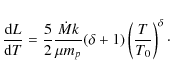
For a steady cooling flow at constant pressure, we would have
![\begin{figure}
\par\includegraphics[width=8.5cm,clip]{12377f13.eps}
\end{figure}](/articles/aa/full_html/2010/05/aa12377-09/img262.png)
|
Figure 13:
The fraction of differential luminosity vs. T0/
|
| Open with DEXTER | |
4.2 Temperature profiles
Perhaps two of the most striking plots from Fig. 6
are subplots J and K, which show a sudden break at
![]() 1
h71-1/2 Gyr. In fact, we find that for the most part
only SCC clusters have a central temperature drop. All 28 SCC clusters
have a central temperature drop and of the eight non-SCC clusters with
a central temperature drop (see Table 3), four (A1650, A2065,
A2142 and A2589) have CCT < 2
h71-1/2 Gyr, putting them on
the border between SCC and WCC clusters. Additionally two (A2142 and
A3667) have well-known cold fronts. The other three appear to be
merging clusters in which a cool core has survived: A0400
(Hudson et al. 2006), A0576 (Dupke et al. 2007b) and A2256
(Sun et al. 2002). It is also clear from
Fig. 6K that the inner temperature profiles of these
eight non-SCC clusters are, for the most part, flatter than those of
the SCC clusters (slope
1
h71-1/2 Gyr. In fact, we find that for the most part
only SCC clusters have a central temperature drop. All 28 SCC clusters
have a central temperature drop and of the eight non-SCC clusters with
a central temperature drop (see Table 3), four (A1650, A2065,
A2142 and A2589) have CCT < 2
h71-1/2 Gyr, putting them on
the border between SCC and WCC clusters. Additionally two (A2142 and
A3667) have well-known cold fronts. The other three appear to be
merging clusters in which a cool core has survived: A0400
(Hudson et al. 2006), A0576 (Dupke et al. 2007b) and A2256
(Sun et al. 2002). It is also clear from
Fig. 6K that the inner temperature profiles of these
eight non-SCC clusters are, for the most part, flatter than those of
the SCC clusters (slope ![]() -0.2). We argue that based on this
fact, studies such as those of Burns et al. (2008) and
Sanderson et al. (2006a), which define CC clusters as clusters with a
central temperature drop, are basically defining CC clusters as
clusters with CCT < 1
h71-1/2 Gyr (SCC clusters in our
sample).
-0.2). We argue that based on this
fact, studies such as those of Burns et al. (2008) and
Sanderson et al. (2006a), which define CC clusters as clusters with a
central temperature drop, are basically defining CC clusters as
clusters with CCT < 1
h71-1/2 Gyr (SCC clusters in our
sample).
Some authors claim the existence of a universal inner temperature
profile for relaxed clusters (e.g. Allen et al. 2001b; Sanderson et al. 2006b),
while others find no such universality (e.g. Vikhlinin et al. 2005). A
universal inner temperature profile suggests that clusters either have
a flat central temperature profile or a drop that scales with
![]() and
and
![]() .
It is clear from Fig. 4L
that we do not see such a universal inner temperature profile.
Figure 14 shows all 64 of our temperature profiles out to
0.1
.
It is clear from Fig. 4L
that we do not see such a universal inner temperature profile.
Figure 14 shows all 64 of our temperature profiles out to
0.1
![]() ,
scaled by
,
scaled by
![]() and
and
![]() .
It is
clear from this figure why we do not see a bimodal distribution in
Fig. 4L. There is a continuous range of slopes from a
20% increase above
.
It is
clear from this figure why we do not see a bimodal distribution in
Fig. 4L. There is a continuous range of slopes from a
20% increase above
![]() (MKW8) to a decrease down to 0.2
(MKW8) to a decrease down to 0.2
![]() (A3526 - Centaurus Cluster). We note that some authors
(e.g. Sanderson et al. 2006a) only use single thermal models at all
radii when constructing temperature profiles. We, however, used
double thermal models for the inner annuli in 14 of our SCC clusters
since the addition of the second thermal component improved the fit
significantly (>99% confidence according to the F test). In
these cases the lower temperature was used, causing a steeper
temperature profile than if a single thermal model had been used.
(A3526 - Centaurus Cluster). We note that some authors
(e.g. Sanderson et al. 2006a) only use single thermal models at all
radii when constructing temperature profiles. We, however, used
double thermal models for the inner annuli in 14 of our SCC clusters
since the addition of the second thermal component improved the fit
significantly (>99% confidence according to the F test). In
these cases the lower temperature was used, causing a steeper
temperature profile than if a single thermal model had been used.
It is interesting to note that in Fig. 4K, there does
seem to be a bimodal distribution in T0/
![]() (albeit
with a large dispersion). This suggests that while the radius of the
gas with
(albeit
with a large dispersion). This suggests that while the radius of the
gas with
![]() does not scale with cluster size, the depth
of the drop does. SCC clusters have a central temperature of
does not scale with cluster size, the depth
of the drop does. SCC clusters have a central temperature of
![]() 0.4
0.4
![]() ,
whereas NCC and WCC clusters have T0
,
whereas NCC and WCC clusters have T0![]()
![]() .
As we discuss in the next section, it is
unclear whether this cool gas is associated with the CF or the central
galaxy. In the case of the former this indicates the coolest major
component of gas allowed by the feedback mechanism. That is,
significant quantities of gas do not cool below
.
As we discuss in the next section, it is
unclear whether this cool gas is associated with the CF or the central
galaxy. In the case of the former this indicates the coolest major
component of gas allowed by the feedback mechanism. That is,
significant quantities of gas do not cool below ![]() 0.4
0.4
![]() .
In the case of the latter, it is consistent with observing
that the mass of the brightest cluster galaxy (BCG) scales with the
cluster mass, so that T0/
.
In the case of the latter, it is consistent with observing
that the mass of the brightest cluster galaxy (BCG) scales with the
cluster mass, so that T0/
![]() is constant. This model
would support the simulations of Burns et al. (2008) who find that the CC
grows with the cluster.
is constant. This model
would support the simulations of Burns et al. (2008) who find that the CC
grows with the cluster.
![\begin{figure}
\par\includegraphics[width=8.5cm,clip]{12377f14.eps}
\end{figure}](/articles/aa/full_html/2010/05/aa12377-09/img265.png)
|
Figure 14: The inner temperature profiles of all 64 HIFLUGCS clusters scaled by virial temperature and radius. The error bars on the measurements have been omitted for clarity. There appears to be a range of slopes rather than a bimodal distribution. |
| Open with DEXTER | |
4.2.1 What causes the central temperature drop?
An old but still ongoing controversy is whether the temperature drop in CC clusters is related to the CF or is simply a reflection of the potential well around the BCG. In the case of the former, the central temperature should be reflected by a modified cooling flow model and should simply depend on the energy factors (energy radiated away, along with input energy from conduction and any feedback mechanism). In the latter case the temperature should reflect the mass of the central galaxy and should be independent of any cooling flow model.One check for possible multitemperature components is the need for a
double thermal model in the central annuli. In the central annulus
(annuli) for 14 of 64 HIFLUGCS
clusters (all SCC clusters), a
double thermal fit was a significantly better fit than a single
thermal model. It is possible, since these are projected temperature
profiles, this is simply due to many temperature components along the
line of sight. Even in this case, the projected temperature
components that dominate are the ones near the cluster center where
the emission is peaked. Whether it is the projected spectra of outer
annuli or truly the need for a double temperature fit to the central
spectra, we take this as evidence of many temperature components in
the region of the emission peak for these clusters. Thus the change
in temperature is rapid in these regions. To explicitly demonstrate
that a double thermal model is consistent with more than two
temperature components we ran simulations of spectra with four and
eight thermal models with temperatures equally spaced between 1 and
2 keV. Fitting these spectra indicates that a double thermal model
can,
at Chandra's energy resolution, fully describe the plasma
emission of the underlying four- or eight- temperature components and
provides the statistically best fit to the spectrum (![]() /d.o.f.
/d.o.f.
![]() 1)
1)![]() . For the eight temperature plasma the returned
temperatures were:
. For the eight temperature plasma the returned
temperatures were:
![]() keV and
keV and
![]() keV. Therefore
we interpret annuli that require two thermal models to contain, at
minimum two thermal components, with a low temperature component
keV. Therefore
we interpret annuli that require two thermal models to contain, at
minimum two thermal components, with a low temperature component ![]() T0.
T0.
Figure 15 shows the modified spectral mass deposition
rate,
![]() versus
versus
![]() .
The
striking thing about this plot is that the two values are very often
consistent with each other, especially for the SCC clusters. Based on
this result, one may naïvely believe that the gas cools to
.
The
striking thing about this plot is that the two values are very often
consistent with each other, especially for the SCC clusters. Based on
this result, one may naïvely believe that the gas cools to
![]() (the lowest temperature for the modified cooling flow model -
see Sect. 2.8) at the rate predicted by the classical cooling
flow model, but does not cool at a significant rate below this
temperature. If this is the case there are two possibilities: (1) the
gas is in thermal equilibrium throughout this range of temperatures or
(2) the gas is rapidly heated from
(the lowest temperature for the modified cooling flow model -
see Sect. 2.8) at the rate predicted by the classical cooling
flow model, but does not cool at a significant rate below this
temperature. If this is the case there are two possibilities: (1) the
gas is in thermal equilibrium throughout this range of temperatures or
(2) the gas is rapidly heated from
![]() to
to
![]() ,
when it reaches
,
when it reaches
![]() .
An alternate explanation is that with
the spectral resolution of the Chandra ACIS, we are unable
to distinguish between gas cooling from
.
An alternate explanation is that with
the spectral resolution of the Chandra ACIS, we are unable
to distinguish between gas cooling from
![]() to
to
![]() and a rapid drop of temperature at the center. That is, the
observation that
and a rapid drop of temperature at the center. That is, the
observation that
![]() could simply be a coincidence.
could simply be a coincidence.
![\begin{figure}
\par\includegraphics[width=8.5cm,clip]{12377f15.eps}
\end{figure}](/articles/aa/full_html/2010/05/aa12377-09/img270.png)
|
Figure 15:
This plot is similar to Fig. 10.
|
| Open with DEXTER | |
Investigating further, we plotted
![]() versus kT0(Fig. 16) for the CC clusters. The blue points are SCC
clusters and the black points are WCC clusters. If the gas cools from
versus kT0(Fig. 16) for the CC clusters. The blue points are SCC
clusters and the black points are WCC clusters. If the gas cools from
![]() to
to
![]() at a rate consistent with a classical
cooling flow (and is somehow stopped at
at a rate consistent with a classical
cooling flow (and is somehow stopped at
![]() ), then we would
expect
), then we would
expect
![]() .
Fig. 16 shows
this to be the case for SCC clusters, however no correlation is found
for WCC clusters. As noted earlier, WCC clusters show little or no
temperature drop at the cluster center. However, when fitted with a
modified spectral mass deposition model, there appear to be
significant quantities of gas down to
.
Fig. 16 shows
this to be the case for SCC clusters, however no correlation is found
for WCC clusters. As noted earlier, WCC clusters show little or no
temperature drop at the cluster center. However, when fitted with a
modified spectral mass deposition model, there appear to be
significant quantities of gas down to ![]() 1/3
1/3
![]() .
The
simplest explanation is that
.
The
simplest explanation is that
![]() is not the correct
model and at the energy resolution of the Chandra ACIS, it
is difficult to distinguish between multitemperature components along
the line-of-sight and a cooling flow model down to
is not the correct
model and at the energy resolution of the Chandra ACIS, it
is difficult to distinguish between multitemperature components along
the line-of-sight and a cooling flow model down to ![]() 1/3
1/3
![]() .
With the spectral resolution of the Chandra ACIS
we cannot draw any strong conclusions, however the results for the SCC
clusters argue for further investigation with higher spectral
resolution instruments to see if this trend of
.
With the spectral resolution of the Chandra ACIS
we cannot draw any strong conclusions, however the results for the SCC
clusters argue for further investigation with higher spectral
resolution instruments to see if this trend of
![]() persists.
persists.
![\begin{figure}
\par\includegraphics[width=8.5cm,clip]{12377f16.eps}
\end{figure}](/articles/aa/full_html/2010/05/aa12377-09/img273.png)
|
Figure 16:
The lower temperature in the
modified cooling flow model (
|
| Open with DEXTER | |
In order to check for the correlation of the central cluster gas with
the central galaxy, we compared the position of the brightest cluster
galaxy (BCG) to the position of the emission peak. We identified the
BCGs from visual inspection of the R-band images of the Second-Epoch
Digitized Sky survey (DSS2, see e.g. http://archive.stsci.edu/dss) and then extracted magnitudes and
redshifts from NED, HyperLeda![]() (Paturel et al. 2003) or the compilation by Andernach & Tago
(see Andernach et al. 2005, for a description). We measured the
position of the BCG by fitting a bidimensional Gaussian on its image,
using the NRAO program
FITSview
(Paturel et al. 2003) or the compilation by Andernach & Tago
(see Andernach et al. 2005, for a description). We measured the
position of the BCG by fitting a bidimensional Gaussian on its image,
using the NRAO program
FITSview![]() . The typical uncertainty was
. The typical uncertainty was
![]() 0
0
![]() 5.
Visual inspection of these images allowed the identification of
usually one, sometimes two or three BCG candidates. In the cases in
which there was more than one BCG candidate, we used the candidate
closest to the X-ray peak. Figure 17 shows the histogram of
distance between the X-ray peak and BCG. The histogram is color
coded: blue for SCC clusters, black for WCC clusters and red for NCC
clusters. The fact that all SCC clusters have a BCG at the center
seems to support the idea that the central temperature drop is related
to the presence of the galaxy. On the other hand, 78% of all HIFLUGCS clusters have a BCG within 12
h71-1 kpc of their
X-ray peak (including 61% and 50% of WCC and NCC clusters
respectively) and
5.
Visual inspection of these images allowed the identification of
usually one, sometimes two or three BCG candidates. In the cases in
which there was more than one BCG candidate, we used the candidate
closest to the X-ray peak. Figure 17 shows the histogram of
distance between the X-ray peak and BCG. The histogram is color
coded: blue for SCC clusters, black for WCC clusters and red for NCC
clusters. The fact that all SCC clusters have a BCG at the center
seems to support the idea that the central temperature drop is related
to the presence of the galaxy. On the other hand, 78% of all HIFLUGCS clusters have a BCG within 12
h71-1 kpc of their
X-ray peak (including 61% and 50% of WCC and NCC clusters
respectively) and ![]() 88% have a BCG within 50
h71-1 kpc.
There is a clear discrepancy between the number of WCC clusters (92%)
and NCC clusters (61%) that have a BCG at the X-ray peak (<50
h71-1 kpc) and those that have cool gas at their center:
33% and 11% respectively. Also as noted earlier the temperature
drop in these clusters is generally smaller than it is for SCC
clusters.
88% have a BCG within 50
h71-1 kpc.
There is a clear discrepancy between the number of WCC clusters (92%)
and NCC clusters (61%) that have a BCG at the X-ray peak (<50
h71-1 kpc) and those that have cool gas at their center:
33% and 11% respectively. Also as noted earlier the temperature
drop in these clusters is generally smaller than it is for SCC
clusters.
Here, we do not present this as evidence that temperature drops are or
are not related to the potential of the BCG. On the one hand, all but
one cluster (A2256) with a central temperature drop have a BCG
cospatial with the X-ray peak (<
12 h71-1 kpc), suggesting that
the temperature drop is related to the BCG. On the other hand, there
are many clusters with a BCG at the center and no central temperature
drop. It appears that regardless of the mechanism that causes the
temperature of the gas in the central region to be below
![]() ,
it is easier to heat the gas (to
,
it is easier to heat the gas (to ![]()
![]() )
in the
central region than to permanently separate it from the dark matter
potential well (i.e. the BCG). Simulations suggest that cluster
mergers can destroy cooling flows (e.g. Burns et al. 2008, and references
therein). It is not clear though that such heating need be
done by something as energetic as a major merger. For instance, A1650
has an almost flat temperature profile and yet no evidence for a
recent major merger (Donahue et al. 2005). Other examples of such
clusters are WCC clusters A2244 (Donahue et al. 2005), A1651 and A1060.
)
in the
central region than to permanently separate it from the dark matter
potential well (i.e. the BCG). Simulations suggest that cluster
mergers can destroy cooling flows (e.g. Burns et al. 2008, and references
therein). It is not clear though that such heating need be
done by something as energetic as a major merger. For instance, A1650
has an almost flat temperature profile and yet no evidence for a
recent major merger (Donahue et al. 2005). Other examples of such
clusters are WCC clusters A2244 (Donahue et al. 2005), A1651 and A1060.
![\begin{figure}
\par\includegraphics[width=8cm,clip]{12377f17.eps}
\end{figure}](/articles/aa/full_html/2010/05/aa12377-09/img274.png)
|
Figure 17:
Histogram of projected
separation of the BCG and X-ray emission peak. The colors
represent: blue - SCC clusters, black - WCC clusters and red - NCC clusters. Most of the clusters ( |
| Open with DEXTER | |
To explore this further we compared the central stellar velocity dispersion of the BCG to the central temperature. The BCG central stellar velocity dispersions were collected from HyperLeda, using mean reported values and standard deviation of the values for the uncertainty. In a few cases, if only one measurement was reported, we used the reported error on the measurement. 16 of our 64 HIFLUGCS clusters (including 8 SCC clusters) did not have any data available. Figure 18 shows BCG central stellar velocity dispersion versus kT0. The points are color coded: SCC-blue, WCC-black and NCC-red. Clusters with a central temperature decline are marked with a circle and clusters without a central temperature drop are marked with a square. The 16 clusters with no data available are omitted, but have the same general distribution in kT0 as the 48 plotted clusters. Even when looking at just the SCC clusters, there seems to be only a weak correlation between the BCG's central velocity dispersion and kT0.
Assuming that our above conjecture is correct, that the gas is
relatively easy to heat without removing it from the center of the
potential, then it appears that the temperature of the central gas is
not generally determined by purely gravitational processes in the
local potential. That is, some heating mechanism heats the gas either
slightly above the local virial temperature in SCC clusters or up to
![]()
![]() in WCC and NCC clusters. We emphasize that the
mechanisms do not have to be the same in all cases (e.g. possible AGN
outbursts or sloshing for SCC and WCC borderline cases and mergers for
NCC clusters). This would explain the large scatter in
Fig. 18. It would also predict that the central gas in
clusters such as A1650 will eventually return to the local virial
temperature in the center. In such a case, in order to maintain
pressure equilibrium with the surrounding gas, the density would
increase dramatically, shortening the CCT and returning the cluster to
the SCC subsample. It is not clear in this model which clusters would
be capable of returning to their SCC status and which ones not.
Perhaps the early major mergers of NCC clusters, as proposed by
Burns et al. (2008), prevent the formation of the large central galaxy
needed to reform the CC. Perhaps once the entropy is increased
enough, the gas cannot cool to the local virial temperature in the
time available. Even when suppressed by magnetic fields, thermal
conduction is still likely to increase rapidly with temperature. Given
that its effect is already argued to be significant
(e.g. Zakamska & Narayan 2003), it may well play a role in preventing cool
cores from being re-established after disruption by mergers in hot
clusters. We suggest that simulations of the formation of CCs
considering different central potentials could help understand which
ones can re-form and which cannot and what physical effects are
important in determining the fate of the central gas.
in WCC and NCC clusters. We emphasize that the
mechanisms do not have to be the same in all cases (e.g. possible AGN
outbursts or sloshing for SCC and WCC borderline cases and mergers for
NCC clusters). This would explain the large scatter in
Fig. 18. It would also predict that the central gas in
clusters such as A1650 will eventually return to the local virial
temperature in the center. In such a case, in order to maintain
pressure equilibrium with the surrounding gas, the density would
increase dramatically, shortening the CCT and returning the cluster to
the SCC subsample. It is not clear in this model which clusters would
be capable of returning to their SCC status and which ones not.
Perhaps the early major mergers of NCC clusters, as proposed by
Burns et al. (2008), prevent the formation of the large central galaxy
needed to reform the CC. Perhaps once the entropy is increased
enough, the gas cannot cool to the local virial temperature in the
time available. Even when suppressed by magnetic fields, thermal
conduction is still likely to increase rapidly with temperature. Given
that its effect is already argued to be significant
(e.g. Zakamska & Narayan 2003), it may well play a role in preventing cool
cores from being re-established after disruption by mergers in hot
clusters. We suggest that simulations of the formation of CCs
considering different central potentials could help understand which
ones can re-form and which cannot and what physical effects are
important in determining the fate of the central gas.
![\begin{figure}
\par\includegraphics[width=8cm,clip]{12377f18.eps}
\end{figure}](/articles/aa/full_html/2010/05/aa12377-09/img275.png)
|
Figure 18: BCG's central velocity dispersion versus kT0. Blue points are SCC clusters, black points are WCC clusters and red points are NCC clusters. Circles signify clusters with a central temperature drop and squares signify clusters without a central temperature drop. The 16 clusters with no BCG velocity dispersion data available span the same range. There appears to be no correlation between the BCG's central velocity dispersion and kT0. |
| Open with DEXTER | |
4.3 BCG separation and mergers
Several works show a special relationship between the cooling activity
in cluster cores and the brightest cluster galaxies located within a
certain projected distance from the X-ray peak, typically
50
h71-1 kpc, to the X-ray peak (see Mittal et al. 2009, for more
details). Given that only eight of our 64 clusters have a
significant (>50
h71-1 kpc) projected separation between
the X-ray peak and BCG suggests that separating the BCG from the gas
is more difficult than simply heating the gas and/or disrupting the
cooling flow. Looking more deeply, the eight clusters with BCG-X-ray
peak separations >50
h71-1 kpc ordered from largest to
smallest are: (1) A3376 - ![]() 939
h71-1 kpc, (2) A0754 -
939
h71-1 kpc, (2) A0754 -
![]() 714
h71-1 kpc, (3) A1367 -
714
h71-1 kpc, (3) A1367 - ![]() 666
h71-1 kpc,
(4) A1736 -
666
h71-1 kpc,
(4) A1736 - ![]() 642
h71-1 kpc, (5) A3667 -
642
h71-1 kpc, (5) A3667 -
![]() 155
h71-1 kpc, (6) A2163 -
155
h71-1 kpc, (6) A2163 - ![]() 128
h71-1 kpc,
(7) A2256 -
128
h71-1 kpc,
(7) A2256 - ![]() 110
h71-1 kpc and (8) A2255 -
110
h71-1 kpc and (8) A2255 -
![]() 72
h71-1 kpc
72
h71-1 kpc![]() . All eight of these
clusters have been identified as merging clusters, A3667 is the only
CC cluster (and it is a borderline CC/NCC cluster) and all except
A1736
have been identified as having a radio halo and/or relic(s) (see
Appendix C for individual references). The appearance of
such diffuse, Mpc scale non-thermal emission is thought to be powered
by major mergers. Of the other 56 clusters, only eight (15%) have
been identified as possibly containing diffuse non-thermal
emission on large scales: A1656, A3562, A85, A133, A401, A2152, A4038
and MKW8. Of these eight, for two (A401 and A2142) the detections
seem unlikely (Giovannini & Feretti 2000), three (A85, A133 and A4038) are
small scale (a few tens of kpc) relics associated with nearby radio
galaxies (e.g. Slee et al. 2001) and one (MKW8) as identified as a
possible relic as seen in the VLA Low-Frequency Sky Survey (VLSS) at
74 MHz (Cohen et al. 2007). Kempner et al. (2004) identified three
classes of radio relics that were fundamentally different. We argue
that in these four cases, the relics are not the large scale Gischt associated with mergers, but AGN-relics. This leaves
only two (4%) unambiguous detections of large scale diffuse radio
emission: the Coma cluster and A3562. Based on the large discrepancy
between the number of clusters with large scale (
. All eight of these
clusters have been identified as merging clusters, A3667 is the only
CC cluster (and it is a borderline CC/NCC cluster) and all except
A1736
have been identified as having a radio halo and/or relic(s) (see
Appendix C for individual references). The appearance of
such diffuse, Mpc scale non-thermal emission is thought to be powered
by major mergers. Of the other 56 clusters, only eight (15%) have
been identified as possibly containing diffuse non-thermal
emission on large scales: A1656, A3562, A85, A133, A401, A2152, A4038
and MKW8. Of these eight, for two (A401 and A2142) the detections
seem unlikely (Giovannini & Feretti 2000), three (A85, A133 and A4038) are
small scale (a few tens of kpc) relics associated with nearby radio
galaxies (e.g. Slee et al. 2001) and one (MKW8) as identified as a
possible relic as seen in the VLA Low-Frequency Sky Survey (VLSS) at
74 MHz (Cohen et al. 2007). Kempner et al. (2004) identified three
classes of radio relics that were fundamentally different. We argue
that in these four cases, the relics are not the large scale Gischt associated with mergers, but AGN-relics. This leaves
only two (4%) unambiguous detections of large scale diffuse radio
emission: the Coma cluster and A3562. Based on the large discrepancy
between the number of clusters with large scale (![]() Mpc) radio
structure that have a large BCG-EP separation and those that do not,
we argue that a large separation of the EP and BCG is a very good
indication a major merger and therefore could be applied as a useful
method for discovering radio halos and radio relics-Gischt.
Mpc) radio
structure that have a large BCG-EP separation and those that do not,
we argue that a large separation of the EP and BCG is a very good
indication a major merger and therefore could be applied as a useful
method for discovering radio halos and radio relics-Gischt.
4.4 WCC clusters
The WCC clusters are an interesting set because they seem to occupy a transition between NCC and SCC clusters. They are defined as having short to moderate CCTs (1.0-7.7 h71-1/2 Gyr), and generally have flat or shallow central temperature drops and a central entropy that is enhanced compared to their SCC cousins. Due to their flat or shallow temperature profile, they are mostly classified as NCC clusters in studies that determine CC clusters by a central temperature drop. Recently Burns et al. (2008) suggested that CC clusters were not necessarily more relaxed than NCC clusters. Since Burns et al. (2008) define CC/NCC classification based on temperature drop, they would classify the WCC clusters as NCC clusters. Could these WCC clusters be the relaxed NCCs? Donahue et al. (2005) studied two radio quiet, relaxed WCC clusters - A1650 and A2244. They conclude that these objects are CC clusters that have had a major AGN outburst, raising the central entropy and temporarily disrupting the CF.In an effort to distinguish between these two possibilities we examined the X-ray morphology of the WCC and NCC clusters. We divided these 36 clusters into four types: (I) relaxed with short CCT (<3 h71-1/2 Gyr), (II) relaxed with moderate/long CCT (>3 h71-1/2 Gyr), (III) disturbed with short CCT (<3 h71-1/2 Gyr), (IV) disturbed with moderate/long CCT (>3 h71-1/2 Gyr). We classify relaxed versus disturbed by visual inspection. We define a relaxed cluster as having: (1) round or elliptical isophotes; (2) the EP at the center of the isophotes and (3) little or no offset between the centers of the different levels of isophotes (little or no sloshing). We note, based on our classification scheme, that all our NCC clusters will be of type II or IV. Our physical interpretation of the four types are: (I) CCs that have been disrupted, but will re-form - their CCTs are too short to be relaxed NCCs, (II) clusters that have not had a recent merger but have had their CC severely disrupted (or destroyed) by a previous major merger (III) clusters that are merging with the core surviving (although it may be destroyed in the future) and (IV) merging clusters in which there was no cool core or the core has been destroyed.
In order to check our categorization based on visual inspection, we plotted the distance between the EP and the X-ray emission weighted center (EWC) (see Hudson et al. 2006, for details on determining the EWC). This method gives a simple way to classify clusters, since disturbed clusters will generally have a larger distance between their EP and EWC than a relaxed clusters. Figure 19 shows the results for the 36 WCC and NCC clusters. Black points indicate the clusters identified as being relaxed and the red points indicate the disturbed clusters. Figure 19 confirms that, in general, the disturbed clusters have a larger separation between the EP and EWC than the relaxed clusters.
![\begin{figure}
\par\includegraphics[width=8cm,clip]{12377f19.eps}
\end{figure}](/articles/aa/full_html/2010/05/aa12377-09/img276.png)
|
Figure 19:
Distance between the X-ray emission peak and
emission weighted center for the 36 WCC and NCC clusters. The black
points are clusters that appear relaxed and the red points are
clusters that appear disturbed. The vertical dashed line separates
clusters with short CCT and long CCT. The dash-dot line divides the
clusters between WCC and NCC. It is clear that in general the
separation of the EP and EWC is larger for the apparently disturbed
clusters. The error on the separation is 4
|
| Open with DEXTER | |
We find seven clusters of type I, six clusters of type II, five clusters of type III and 18 clusters of type IV. By the definition of Burns et al. (2008), these 36 clusters are clusters that will never form a CC. We argue, however, given the short cooling time of the clusters of type I, it is unlikely that their CCT will never drop below 1 h71-1/2 Gyr, which in turn implies they will also have a central temperature drop. 39% of the WCC clusters are of this type and are perhaps a special type of SCC cluster that experienced an anomalous event that has temporarily disrupted the strong cool core (e.g. raised the central temperature, entropy and cooing time).
We acknowledge that a more sophisticated method should be employed
when determining whether a cluster is relaxed or not. However based
on preliminary results, unless WCC clusters (especially those with
short CCT) are fundamentally different from SCC clusters, some of them
will become SCC clusters. That is, unless there is a process that
keeps their CCT > 1
h71-1/2 Gyr and their
temperature-profile flat, the gas in the core will cool below
![]() and the CCT will drop below unity.
and the CCT will drop below unity.
5 Conclusions
We provide the most detailed systematic view into X-ray cores of galaxy clusters to date. We find that the best method to determine whether a cluster is a cool-core (CC) cluster is with the central cooling time (CCT). We divide clusters into three types: strong cool-core (SCC), weak cool-core (WCC or transition) and non-cool-core clusters. SCC are defined as having very short CCT (<1 h71-1/2 Gyr) and are characterized by low central entropy (Based on the above classification, our main conclusions are:
- 1.
- In our flux-limited statistically complete sample, we find 72% of the clusters are CC clusters with 44% of the clusters being SCC clusters and 28% being WCC clusters.
- 2.
- For intermediate redshift clusters (where radii as small as
0.4% r500 cannot be resolved), we find that
and
scaled
are the best proxies for CCT. In general
is better, but needs to be standardized before it is used.
We suggest using
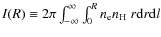 with
a possible value of
with
a possible value of
 h71-2 cm-3.
- 3.
- For high redshift clusters (clusters with very few counts), we
find that cuspiness is the most useful proxy. However, it suffers
from a large scatter in the relation to CCT, so precise
categorizations can be difficult. Preliminary results suggest that
a concentration parameter (
 kpc)/
kpc)/
 kpc)), as
suggested by Santos et al. (2008), may serve as the best proxy for
distant clusters.
kpc)), as
suggested by Santos et al. (2008), may serve as the best proxy for
distant clusters.
- 4.
- Dividing our representative sample into four redshift bins, we
find it unlikely that the discrepancy between spectral mass
deposition rate (
)
and classical mass deposition
rate (
)
is due to the fact that CCs formed
very recently. The probability that the lowest- and the
highest-redshift clusters with non-zero forward-evolved mass
deposition rates come from the same population is extremely low
(<
 ). This requires the discrepancy to be explained by some
heating method.
). This requires the discrepancy to be explained by some
heating method.
- 5.
- There is no evidence found in our work for a universal central
temperature profile as claimed previously for smaller samples. This
suggests that the radius of the cool gas is not universal. As seen
in Table 2, the radius within which the temperature falls
below
differs from cluster to cluster.
- 6.
- We find the majority (
 78%) of HIFLUGCS clusters,
including 100% of the SCC clusters, 61% of the WCC clusters and
50% of the NCC clusters, have a BCG within 12
h71-1 kpc of
the X-ray emission peak. This number increases to 88% for a
distance of 50
h71-1 kpc. We find that seven out of eight
clusters with the BCG-EP separation >50
h71-1 kpc have
Mpc scale radio emission (halo or relic-Gischt) versus only
two of the remaining 56 with a BCG very close to the EP.
78%) of HIFLUGCS clusters,
including 100% of the SCC clusters, 61% of the WCC clusters and
50% of the NCC clusters, have a BCG within 12
h71-1 kpc of
the X-ray emission peak. This number increases to 88% for a
distance of 50
h71-1 kpc. We find that seven out of eight
clusters with the BCG-EP separation >50
h71-1 kpc have
Mpc scale radio emission (halo or relic-Gischt) versus only
two of the remaining 56 with a BCG very close to the EP.
- 7.
- There is a weak correlation between the SCC central temperature
and the cooling of the gas as predicted by the cooling flow model.
We also find no correlation between the SCC central temperature and
the central velocity dispersion of the BCG. We interpret this,
along with the result that so many clusters have a BCG at their
peak, as indicating that the central temperature of the gas is
influenced by heating, which occurs differently in different
clusters. Therefore, the central temperature is not simply
reflective of the central potential well or the expected cooling
rate from
 to
to
 ,
but requires more complex
physics.
,
but requires more complex
physics.
- 8.
- We find that <39% of the WCC clusters which are relaxed also
have relatively short cooling times (
 Gyr). We argue that these clusters are similar to SCC
clusters but have had an event that temporarily disrupted the cool
core, raising the core temperature, entropy and cooling time.
Gyr). We argue that these clusters are similar to SCC
clusters but have had an event that temporarily disrupted the cool
core, raising the core temperature, entropy and cooling time.
The authors wish to thank D. A. Buote, T. E. Clarke, M. Markevitch and A. Vikhlinin for providing proprietary data before it was publicly available. We would like to thank E. Murphy for providing pointed radio measurements offor several clusters. We thank E. Blanton, H. Böhringer, Y. Ikebe, E. Pierpaoli, S. Randall, P. Schuecker, and G. Sivakoff for help in the early stages of this work. We would like to thank R. Smith for providing the data for the APEC model. We thank the referee for a beneficial feedback and James Wicker for useful correspondence. T. H. R. and D. S. H. acknowledge support from the Deutsche Forschungsgemeinschaft through Emmy Noether research grant RE 1462/2. R. M. acknowledges support from the Deutsche Forschungsgemeinschaft through the Schwerpunkt Program 1177 (RE 1462/4). H. A. acknowledges financial support from CONACyT under grants 50921-F and 81356, and partial support from the Transregional Collaborative Research Center TRR33 ``The Dark Universe''. P. E. J. N. acknowledges support from NASA grant NAS8-03060. C. L. S. was supported in part by NASA Chandra grants GO7-8129X and AR7-8012X and NASA XMM-Newton grant NNX06AE76G. This research has made use of the NASA/IPAC Extragalactic Database (NED) which is operated by the Jet Propulsion Laboratory, California Institute of Technology, under contract with the National Aeronautics and Space Administration. We acknowledge the usage of the HyperLeda database (http://leda.univ-lyon1.fr).
References
- Akritas, M. G., & Bershady, M. A. 1996, ApJ, 470, 706
- Allen, S. W., Fabian, A. C., Johnstone, R. M., Arnaud, K. A., & Nulsen, P. E. J. 2001a, MNRAS, 322, 589
- Allen, S. W., Schmidt, R. W., & Fabian, A. C. 2001b, MNRAS, 328, L37
- Andernach, H., Tago, E., Einasto, M., Einasto, J., & Jaaniste, J. 2005, in Nearby Large-Scale Structures and the Zone of Avoidance, ed. A. P. Fairall, & P. A. Woudt, ASP Conf. Ser., 329, 283
- Ashman, K. M., Bird, C. M., & Zepf, S. E. 1994, AJ, 108, 2348
- Bagchi, J., Durret, F., Neto, G. B. L., & Paul, S. 2006, Science, 314, 791
- Bauer, F. E., Fabian, A. C., Sanders, J. S., Allen, S. W., & Johnstone, R. M. 2005, MNRAS, 359, 1481
- Baumgartner, W. H., & Mushotzky, R. F. 2006, ApJ, 639, 929
- Belsole, E., Birkinshaw, M., & Worrall, D. M. 2005, MNRAS, 358, 120
- Bîrzan, L., McNamara, B. R., Nulsen, P. E. J., Carilli, C. L., & Wise, M. W. 2008, ApJ, 686, 859
- Bîrzan, L., Rafferty, D. A., McNamara, B. R., Wise, M. W., & Nulsen, P. E. J. 2004, ApJ, 607, 800
- Blanton, E. L., Sarazin, C. L., McNamara, B. R., & Wise, M. W. 2001, ApJ, 558, L15
- Böhringer, H., Burwitz, V., Zhang, Y.-Y., Schuecker, P., & Nowak, N. 2005, ApJ, 633, 148
- Bonamente, M., Nevalainen, J., & Lieu, R. 2007, ApJ, 668, 796
- Bridle, A. H., & Fomalont, E. B. 1976, A&A, 52, 107
- Buote, D. A., & Lewis, A. D. 2004, ApJ, 604, 116
- Burns, J. O., Hallman, E. J., Gantner, B., Motl, P. M., & Norman, M. L. 2008, ApJ, 675, 1125
- Cavagnolo, K. W., Donahue, M., Voit, G. M., & Sun, M. 2009, ApJS, 182, 12
- Cavaliere, A., & Fusco-Femiano, R. 1976, A&A, 49, 137
- Chatzikos, M., Sarazin, C. L., & Kempner, J. C. 2006, ApJ, 643, 751
- Chen, Y., Reiprich, T. H., Böhringer, H., Ikebe, Y., & Zhang, Y.-Y. 2007, A&A, 466, 805
- Clarke, T. E., & Ensslin, T. A. 2006, AJ, 131, 2900
- Clarke, T. E., Blanton, E. L., & Sarazin, C. L. 2004, ApJ, 616, 178
- Cohen, A. S., Lane, W. M., Cotton, W. D., et al. 2007, AJ, 134, 1245
- Condon, J. J., Cotton, W. D., Greisen, E. W., et al. 1998, AJ, 115, 1693
- Cortese, L., Gavazzi, G., Boselli, A., Iglesias-Paramo, J., & Carrasco, L. 2004, A&A, 425, 429
- Cortese, L., Gavazzi, G., Boselli, A., et al. 2006, A&A, 453, 847
- Cowie, L. L., & Binney, J. 1977, ApJ, 215, 723
- Crawford, C. S., Sanders, J. S., & Fabian, A. C. 2005, MNRAS, 361, 17
- De Grandi, S., & Molendi, S. 2002, ApJ, 567, 163
- de Plaa, J., Kaastra, J. S., Tamura, T., et al. 2004, A&A, 423, 49
- Dennis, T. J., & Chandran, B. D. G. 2005, ApJ, 622, 205
- Donahue, M. 2007, in Heating versus Cooling in Galaxies and Clusters of Galaxies, ESO Astrophysics Symposia, ed. H. Böhringer, G. W. Pratt, A. Finoguenov, & P. Schuecker (Heidelberg, Berlin: Springer-Verlag), 20
- Donahue, M., Voit, G. M., O'Dea, C. P., Baum, S. A., & Sparks, W. B. 2005, ApJ, 630, L13
- Donnelly, R. H., Forman, W., Jones, C., et al. 2001, ApJ, 562, 254
- Drinkwater, M. J., Gregg, M. D., & Colless, M. 2001, ApJ, 548, L139
- Dunn, R. J. H., & Fabian, A. C. 2006, MNRAS, 373, 959
- Dunn, R. J. H., & Fabian, A. C. 2008, ArXiv e-prints, 801
- Dupke, R., White, III, R. E., & Bregman, J. N. 2007a, ApJ, 671, 181
- Dupke, R. A., Mirabal, N., Bregman, J. N., & Evrard, A. E. 2007b, ApJ, 668, 781
- Edge, A. C. 2001, MNRAS, 328, 762
- Evrard, A. E., Metzler, C. A., & Navarro, J. F. 1996, ApJ, 469, 494
- Fabian, A. C., & Nulsen, P. E. J. 1977, MNRAS, 180, 479
- Fabian, A. C., & Nulsen, P. E. J. 1979, MNRAS, 186, 783
- Fabian, A. C., Sanders, J. S., Ettori, S., et al. 2001, MNRAS, 321, L33
- Feretti, L., Böhringer, H., Giovannini, G., & Neumann, D. 1997, A&A, 317, 432
- Feretti, L., Dallacasa, D., Govoni, F., et al. 1999, A&A, 344, 472
- Feretti, L., & Giovannini, G. 1994, A&A, 281, 375
- Feretti, L., Fusco-Femiano, R., Giovannini, G., & Govoni, F. 2001, A&A, 373, 106
- Finoguenov, A., Henriksen, M. J., Briel, U. G., de Plaa, J., & Kaastra, J. S. 2004, ApJ, 611, 811
- Finoguenov, A., Henriksen, M. J., Miniati, F., Briel, U. G., & Jones, C. 2006, ApJ, 643, 790
- Finoguenov, A., Reiprich, T. H., & Böhringer, H. 2001, A&A, 368, 749
- Fujita, Y., Sarazin, C. L., Kempner, J. C., et al. 2002, ApJ, 575, 764
- Fujita, Y., Sarazin, C. L., Reiprich, T. H., et al. 2004, ApJ, 616, 157
- Gavazzi, G., & Trinchieri, G. 1983, ApJ, 270, 410
- Giacintucci, S., Venturi, T., Brunetti, G., et al. 2005, A&A, 440, 867
- Giovannini, G., & Feretti, L. 2000, New Astron., 5, 335
- Giovannini, G., Tordi, M., & Feretti, L. 1999, New Astron., 4, 141
- Gonzalez, A. H., Zabludoff, A. I., Zaritsky, D., & Dalcanton, J. J. 2000, ApJ, 536, 561
- Guo, F., & Oh, S. P. 2008, MNRAS, 384, 251
- Henriksen, M. J., & Tittley, E. R. 2002, ApJ, 577, 701
- Henriksen, M. J., & White, III, R. E. 1996, ApJ, 465, 515
- Henry, J. P., Finoguenov, A., & Briel, U. G. 2004, ApJ, 615, 181
- Hudson, D. S., & Reiprich, T. H. 2007, in Heating versus Cooling in Galaxies and Clusters of Galaxies, ed. H. Böhringer, G. W. Pratt, A. Finoguenov, & P. Schuecker, 42
- Hudson, D. S., Reiprich, T. H., Clarke, T. E., & Sarazin, C. L. 2006, A&A, 453, 433
- Ikebe, Y., Reiprich, T. H., Böhringer, H., Tanaka, Y., & Kitayama, T. 2002, A&A, 383, 773
- Johnstone, R. M., Fabian, A. C., Morris, R. G., & Taylor, G. B. 2005, MNRAS, 356, 237
- Kaastra, J. S., Ferrigno, C., Tamura, T., et al. 2001, A&A, 365, L99
- Kalberla, P. M. W., Burton, W. B., Hartmann, D., et al. 2005, A&A, 440, 775
- Kassim, N. E., Clarke, T. E., Enßlin, T. A., Cohen, A. S., & Neumann, D. M. 2001, ApJ, 559, 785
- Kempner, J. C., Blanton, E. L., Clarke, T. E., et al. 2004, in The Riddle of Cooling Flows in Galaxies and Clusters of galaxies, ed. T. Reiprich, J. Kempner, & N. Soker, 335
- Kempner, J. C., & David, L. P. 2004, ApJ, 607, 220
- Kempner, J. C., Sarazin, C. L., & Ricker, P. M. 2002, ApJ, 579, 236
- Kuntz, K. D. 2001, Ph.D. Thesis, NASA Goddard Space Flight Center
- Lea, S. M., Silk, J., Kellogg, E., & Murray, S. 1973, ApJ, 184, L105
-
 okas, E. L., Wojtak, R., Gottlöber, S., Mamon, G. A., &
Prada, F. 2006, MNRAS, 367, 1463
okas, E. L., Wojtak, R., Gottlöber, S., Mamon, G. A., &
Prada, F. 2006, MNRAS, 367, 1463
- Machalski, J., & Condon, J. J. 1999, ApJS, 123, 41
- Makishima, K., Ezawa, H., Fukuzawa, Y., et al. 2001, PASJ, 53, 401
- Mann, H. B., & Whitney, D. R. 1947, Annals of Mathematical Statistics, 18, 50
- Markevitch, M., & Vikhlinin, A. 2001, ApJ, 563, 95
- Markevitch, M., Forman, W. R., Sarazin, C. L., & Vikhlinin, A. 1998, ApJ, 503, 77
- Markevitch, M., Ponman, T. J., Nulsen, P. E. J., et al. 2000, ApJ, 541, 542
- Markevitch, M., Vikhlinin, A., & Mazzotta, P. 2001, ApJ, 562, L153
- Mathews, W. G., & Bregman, J. N. 1978, ApJ, 224, 308
- Mathews, W. G., Faltenbacher, A., & Brighenti, F. 2006, ApJ, 638, 659
- Mazzotta, P., Brunetti, G., Giacintucci, S., Venturi, T., & Bardelli, S. 2004, J. Korean Astron. Soc., 37, 381
- McNamara, B. R., & O'Connell, R. W. 1989, AJ, 98, 2018
- McNamara, B. R., Wise, M. W., Nulsen, P. E. J., et al. 2001, ApJ, 562, L149
- Mewe, R., Gronenschild, E. H. B. M., & van den Oord, G. H. J. 1985, A&AS, 62, 197
- Mewe, R., Lemen, J. R., & van den Oord, G. H. J. 1986, A&AS, 65, 511
- Mittal, R., Hudson, D. S., Reiprich, T. H., & Clarke, T. 2009, A&A, 501, 835
- Molendi, S., & Pizzolato, F. 2001, ApJ, 560, 194
- Morris, R. G., & Fabian, A. C. 2005, MNRAS, 358, 585
- Mushotzky, R. F., & Szymkowiak, A. E. 1988, in NATO ASIC Proc. 229: Cooling Flows in Clusters and Galaxies, ed. A. C. Fabian, 53
- Nevalainen, J., Oosterbroek, T., Bonamente, M., & Colafrancesco, S. 2004, ApJ, 608, 166
- Nulsen, P. E. J., McNamara, B. R., Wise, M. W., & David, L. P. 2005, ApJ, 628, 629
- Oegerle, W. R., Cowie, L., Davidsen, A., et al. 2001, ApJ, 560, 187
- O'Hara, T. B., Mohr, J. J., Bialek, J. J., & Evrard, A. E. 2006, ApJ, 639, 64
- Paturel, G., Petit, C., Prugniel, P., et al. 2003, A&A, 412, 45
- Peterson, J. R., Kahn, S. M., Paerels, F. B. S., et al. 2003, ApJ, 590, 207
- Peterson, J. R., Paerels, F. B. S., Kaastra, J. S., et al. 2001, A&A, 365, L104
- Rafferty, D. A., McNamara, B. R., Nulsen, P. E. J., & Wise, M. W. 2006, ApJ, 652, 216
- Reiprich, T. H. 2006, A&A, 453, L39
- Reiprich, T. H., & Böhringer, H. 2002, ApJ, 567, 716
- Reiprich, T. H., & Hudson, D. S. 2007, in Heating versus Cooling in Galaxies and Clusters of Galaxies, ed. H. Böhringer, G. W. Pratt, A. Finoguenov, & P. Schuecker, 381
- Reiprich, T. H., Hudson, D. S., Zhang, Y. ., et al. 2009, A&A, 501, 899
- Reiprich, T. H., Sarazin, C. L., Kempner, J. C., & Tittley, E. 2004, ApJ, 608, 179
- Roettiger, K., Burns, J. O., & Stone, J. M. 1999, ApJ, 518, 603
- Rossetti, M., Ghizzardi, S., Molendi, S., & Finoguenov, A. 2007, A&A, 463, 839
- Ruszkowski, M., Brüggen, M., & Begelman, M. C. 2004, ApJ, 611, 158
- Sakelliou, I., Peterson, J. R., Tamura, T., et al. 2002, A&A, 391, 903
- Sakelliou, I., & Ponman, T. J. 2004, MNRAS, 351, 1439
- Sanders, J. S., & Fabian, A. C. 2002, MNRAS, 331, 273
- Sanders, J. S., Fabian, A. C., Allen, S. W., et al. 2008, MNRAS, 385, 1186
- Sanderson, A. J. R., Finoguenov, A., & Mohr, J. J. 2005, ApJ, 630, 191
- Sanderson, A. J. R., Ponman, T. J., & O'Sullivan, E. 2006a, MNRAS, 372, 1496
- Sanderson, A. J. R., Ponman, T. J., & O'Sullivan, E. 2006b, MNRAS, 372, 1496
- Santos, J. S., Rosati, P., Tozzi, P., et al. 2008, A&A, 483, 35
- Sato, K., Yamasaki, N. Y., Ishida, M., et al. 2007, PASJ, 59, 299
- Slee, O. B., & Roy, A. L. 1998, MNRAS, 297, L86
- Slee, O. B., Roy, A. L., Murgia, M., Andernach, H., & Ehle, M. 2001, AJ, 122, 1172
- Smith, R. K., & Brickhouse, N. S. 2000, in ed. S. J. Arthur, N. S. Brickhouse, & J. Franco, Rev. Mex. Astron. Astrof. Conf. Ser., 9, 134
- Smith, R. K., Brickhouse, N. S., Liedahl, D. A., & Raymond, J. C. 2001, in Spectroscopic Challenges of Photoionized Plasmas, ed. G. Ferland, & D. W. Savin, ASP Conf. Ser., 247, 161
- Sun, M., & Vikhlinin, A. 2005, ApJ, 621, 718
- Sun, M., Murray, S. S., Markevitch, M., & Vikhlinin, A. 2002, ApJ, 565, 867
- Sun, M., Vikhlinin, A., Forman, W., Jones, C., & Murray, S. S. 2005, ApJ, 619, 169
- Takizawa, M., Sarazin, C. L., Blanton, E. L., & Taylor, G. B. 2003, ApJ, 595, 142
- Tamura, T., Bleeker, J. A. M., Kaastra, J. S., Ferrigno, C., & Molendi, S. 2001a, A&A, 379, 107
- Tamura, T., Kaastra, J. S., Peterson, J. R., et al. 2001b, A&A, 365, L87
- Tittley, E. R., & Henriksen, M. 2001, ApJ, 563, 673
- Venturi, T., Bardelli, S., Morganti, R., & Hunstead, R. W. 2000, MNRAS, 314, 594
- Vikhlinin, A., Burenin, R., Forman, W. R., et al. 2007, in Heating versus Cooling in Galaxies and Clusters of Galaxies, ed. H. Böhringer, G. W. Pratt, A. Finoguenov, & P. Schuecker, 48
- Vikhlinin, A., Markevitch, M., & Murray, S. S. 2001a, ApJ, 551, 160
- Vikhlinin, A., Markevitch, M., & Murray, S. S. 2001b, ApJ, 549, L47
- Vikhlinin, A., Markevitch, M., Murray, S. S., et al. 2005, ApJ, 628, 655
- Vikhlinin, A., Burenin, R. A., Ebeling, H., et al. 2009, ApJ, 692, 1033
- Voit, G. M., Cavagnolo, K. W., Donahue, M., et al. 2008, ApJ, 681, L5
- Werner, N., Kaastra, J. S., Takei, Y., et al. 2007, A&A, 468, 849
- Wilcoxon, F. 1945, Biometrics, 1, 80
- Willson, M. A. G. 1970, MNRAS, 151, 1
- Xu, H., Kahn, S. M., Peterson, J. R., et al. 2002, ApJ, 579, 600
- Yamasaki, N. Y., Ohashi, T., & Furusho, T. 2002, ApJ, 578, 833
- Zakamska, N. L., & Narayan, R. 2003, ApJ, 582, 162
- Zappacosta, L., Buote, D. A., Gastaldello, F., et al. 2006, ApJ, 650, 777
Online Material
Appendix A: Calculating central density for a double
model
Starting from the definition of the normalization of the APEC model (Mewe et al. 1985; Smith et al. 2001; Mewe et al. 1986; Smith & Brickhouse 2000)
and taking
![]() with
with
![]() ,
(calculated individually, but generally
,
(calculated individually, but generally ![]() 1.2),
1.2),
where the terms are defined as in Eq. (9). For a double
![\begin{displaymath}n(r) = \left[ n_{01}^{2} \left( 1 + \left( \frac{r}{r_{\rm c_...
...} \right)^{2} \right)^{-3\beta_{2}} \right]^{\frac{1}{2}}\cdot
\end{displaymath}](/articles/aa/full_html/2010/05/aa12377-09/img288.png)
The unabsorbed
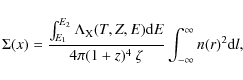
where r2 = x2 + l2 and
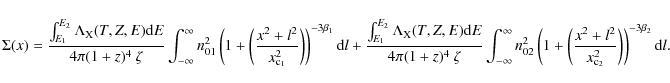
Solving the integral gives the standard expression for the double
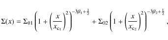
where
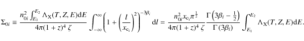
Therefore,
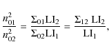
where LIi and
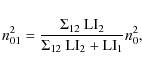
and
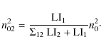
Inserting these values into Eq. (A.2) to find an expression for n(r) in terms of n0, we get
![\begin{displaymath}n(r) =\frac{n_{0}}{\sqrt{\Sigma_{12}\:{\rm LI}_{2}+ {\rm LI}_...
...{2}}} \right)^{2} \right)^{-3\beta_{2}} \right]^{\frac{1}{2}}.
\end{displaymath}](/articles/aa/full_html/2010/05/aa12377-09/img299.png)
Inserting this expression of n(r) into Eq. (A.1) and solving for n0, we recover Eq. (12).
Appendix B: K
 calculations
From the definition of surface brightness (Eq. (A.3)), a
cluster at redshift z, of a region with an angular radius x, has
an integrated surface brightness (or Flux
![]() )
between
energies E1 and E2:
)
between
energies E1 and E2:
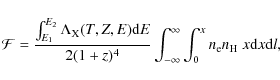
where
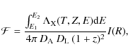
where
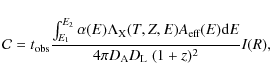
where
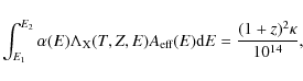
|
(B.4) |
so that
Using an on-axis Chandra ARF and RMF, we determined
|
(B.6) |
Appendix C: Notes on individual clusters
C.1 A0085
This cluster appears to have two subclumps, one near the center and one further to the south (Kempner et al. 2002). In determining the temperature profile and global cluster temperature the latter was excluded. This SCC cluster hosts a well-studied radio relic, which is close to but not connected to the central radio galaxy (e.g. Slee et al. 2001). The central region of this cluster requires a double thermal model out toC.2 A0119
This is possibly a merging cluster, which shows elongation towards the northeast. The X-ray peak of this NCC cluster, which does not dominate the surface brightness, has a cD galaxy cospatial with it. The cluster contains three wide-angle-tailed (WAT) radio galaxies which may be interacting with the ICM (e.g. Feretti et al. 1999).C.3 A0133
Central regions of this cluster show an east-west elongation. An in-depth study with XMM and Chandra by Fujita et al. (2004,2002) revealed an X-ray tongue extending northwest. This SCC cluster hosts a radio relic, that is close to but not connected to the central radio galaxy (e.g. Slee et al. 2001). The central region of this cluster requires a double thermal model out toC.4 NGC 0507 group
The overall X-ray spectrum of this group shows a suspicious hard tail. An additional powerlaw component was included in the overall temperature fit. It is possible that the hard tail is due to unresolved low mass X-ray binaries (LMXBs), although the central region (C.5 A0262
The spectral fits to the inner regions are poor (C.6 A0400
This cluster hosts the double radio source 3C75 within its center and shows evidence of merging (Hudson et al. 2006). As noted in Hudson et al. (2006), the hydrogen column density is higher than measured in the radio (C.7 A0399
This cluster is near to A401 and shows evidence of interaction with A401 (e.g. Sakelliou & Ponman 2004). The temperature profile of this cluster peaks at the X-ray center.C.8 A0401
See also A0399. This cluster may host a radio halo (Giovannini et al. 1999). We included an early observation (before 2001), since the later observation was offset, with the cluster center in the corner of a CCD. The BCG closest to the X-ray peak isC.9 A3112
Although the background flaring seen in some observations was removed, the effect seems to have broadened a fluorescence line. This can be seen in the fit to the overall cluster spectrum (atC.10 NGC 1399/Fornax cluster
This nearby SCC cluster has two X-ray peaks cospatial with NGC 1399 and NGC 1404. The X-ray peak is taken to be cospatial with the BCG NGC 1399. The peak on NGC 1404 was removed for spatial and spectral analysis. Fornax appears to be an outlier in six of the plots of parameters versus CCT in which it has an anomalously low value for its CCT. These parameters are: (1)C.11 2A0335+096
This cluster, along with A0478 and NGC 1550, has a significantly higher
hydrogen column density than measured at radio wavelengths
(
![]() cm-2 Kalberla et al. 2005). We fit
all spectra with the column density free. For the fit to the overall
spectrum we find
cm-2 Kalberla et al. 2005). We fit
all spectra with the column density free. For the fit to the overall
spectrum we find
![]() cm-2. This
cluster has two major galaxies near the X-ray peak, which resides
between the two of them (
cm-2. This
cluster has two major galaxies near the X-ray peak, which resides
between the two of them (![]() 10
h71-1 kpc from the closest).
Of the 16 clusters in which no information about the BCG central
velocity dispersion is available, this cluster has the shortest CCT.
The central region of this cluster requires a double thermal model out
to
10
h71-1 kpc from the closest).
Of the 16 clusters in which no information about the BCG central
velocity dispersion is available, this cluster has the shortest CCT.
The central region of this cluster requires a double thermal model out
to ![]() 38
38
![]() (
(![]() 26
h71-1 kpc).
26
h71-1 kpc).
C.12 IIIZw54
IIIZw54 is a pair of galaxies near the center of a poor galaxy group. We used a 6C.13 A3158
okas et al. (2006) report A3158 as a relaxed cluster based on the velocity dispersion of the galaxies. The X-ray emission appears to be elliptical and there are two cDs near the cluster center, one of which lies at the X-ray peak. This cluster definitely does not have a bright core, with a central density of onlyC.14 A0478
This cluster, along with 2A0335+096 and NGC 1550, has a significantly higher hydrogen column density than measured in the radio (C.15 NGC 1550 group
This cluster, along with 2A0335+096 and A0478, has a significantly higher hydrogen column density than measured in the radio (C.16 EXO0422-086/RBS 0540
The short observation of this SCC cluster indicates a round, centrally peaked cluster with a moderate central temperature drop. The BL Lac object EXO 0423.4-0840 at the center of this cluster was studied by Belsole et al. (2005). This is one of sixteen clusters for which no data about the BCG central velocity dispersion are available.C.17 A3266
This cluster has a very low background scaling factor; therefore an additional unfolded powerlaw component was included in the spectral fits to account for any residual particle background. Reading in the background as a corfile (i.e. a second background component with an adjustable scaling factor), the overall best-fit temperature is found to be consistent with our result including an unfolded powerlaw. Henriksen & Tittley (2002); Finoguenov et al. (2006) presented detailed analyses of this merging system.C.18 A0496
The high abundances in the central region of this cluster are better fit with a VAPEC model, however since this did not change the best-fit values of temperature, solar ratios were used for simplicity. A double thermal model greatly improved the fits to spectra in annuli out to 0C.19 A3376
This cluster was fit with an unfolded powerlaw component to account for possible low-level flares in both observations. This cluster appears highly disturbed in the X-ray with a strong elongation along the east-west direction. Bagchi et al. (2006) report the existence of double relics, one to the east of the cluster center and one to the west. Nevalainen et al. (2004) found a diffuse, hard excess with the BeppoSAX PDS at 2.7C.20 A3391
The short observation of this NCC cluster shows an elliptical shaped ICM with a BCG cospatial with the emission peak. Tittley & Henriksen (2001) discovered a filament between A3391 and the nearby cluster A3395.C.21 A3395s
This cluster is very close to and may be interacting with A3395e. A3395e was excluded from all extended analysis. Donnelly et al. (2001) claim A3395s and A3395e are near first core passage.C.22 A0576
Kempner & David (2004) originally presented an analysis of the Chandra data. Dupke et al. (2007b) presented a detailed analysis of the XMM-Newton and Chandra data suggesting that it is a line-of-sight merger. The X-ray image seems somewhat perturbed with elliptical isophotes with alternating NW-SE shifted centers, reminiscent of sloshing, already noted by Kempner & David (2004). The BCG isC.23 A0754
This irregularly shaped cluster hosts a halo and relic (Kassim et al. 2001). Henry et al. (2004) presented a detailed analysis of this merging system using the XMM-Newton observation. Only the pre-2001 Chandra observation is used, since it was the only one that contained the cluster core. More recent observation have been made but do not cover the cluster center and therefore are not useful for core studies. The BCG for this cluster isC.24 A0780/Hydra-A cluster
This cluster is known to have a massive central AGN outburst (Nulsen et al. 2005).C.25 A1060
This WCC cluster is also known as the Hydra cluster. Sato et al. (2007) recently presented a Suzaku observation of this cluster. This cluster has two bright galaxies near the core, one of which is cospatial with X-ray peak. Both galaxies have a clearly visible diffuse X-ray component (Yamasaki et al. 2002).C.26 A1367
Due to the short exposure time and lack of a bright core, we used a 12C.27 MKW4
A single thermal model is a poor fit to this high metalicity center. Although a second thermal model does provide an improvement, freeing the ratio of elements for a single thermal model provides the best-fit. Since freeing the abundance ratios does not change the overall best-fit temperatures of the annuli, solar ratios with a single thermal model were used for simplicity.C.28 ZwCl 1215.1+0400
The short observation of this NCC cluster, shows a round cluster with no bright central peak and an elliptical BCG located at the X-ray emission peak. This is one of the sixteen clusters for which no data about the BCG central velocity dispersion are available. The BCG of this clusters is alsoC.29 NGC 4636 group
This nearby group contains extended nonthermal emission in the central region extending outC.30 A3526/Centaurus cluster
This is a well-studied, prototypical CC cluster, with a central temperature drop (having the largest fractional drop,C.31 A1644
As with A0085, this SCC cluster shows evidence of merging, with the existence of a double X-ray peak. Reiprich et al. (2004) analyzed the XMM EPIC observation of this cluster. They found the flux of the northern (smaller) subclump is below the HIFLUGCS flux limit whereas the flux of the southern (larger) subclump is above the flux limit. Therefore for purposes of this analysis the smaller subclump was excluded from spatial and spectral analysis. Additionally Reiprich et al. (2004) found evidence that the smaller sub-clump was being stripped as it passes through the ICM. This is one of sixteen clusters in which the central velocity dispersion of the BCG is unavailable. The central region of this cluster requires a double thermal model out toC.32 A1650
This CC cluster hosts a radio quiet cD galaxy (Donahue et al. 2005). Mittal et al. (2009) find an upper-limit to the bolometric radio luminosity ofC.33 A1651
As with A1650, Donahue et al. (2005) claim this is a radio quiet CC cluster, however Mittal et al. (2009) detect central radio emission with a bolometric luminosity ofC.34 A1656/Coma cluster
This well-studied NCC cluster appears to be involved in a merger with a group. This cluster hosts the first detected radio halo (Willson 1970).C.35 NGC 5044 troup
The spectra for the inner regions of this group are not well fit by a single thermal model (C.36 A1736
This NCC cluster is a member of the Shapley Supercluster. Due to the short exposure time and lack of a bright core, the X-ray peak was found by smoothing the image with aC.37 A3558
This WCC cluster is located in the core of the Shapley Supercluster. The observation was heavily flared, and even after a conservative cleaning of the light curve there was evidence of some low-level flaring in the back-illuminated chips. Rossetti et al. (2007) presented the XMM and Chandra analysis of this cluster, concluding that it had a cool core that had survived a merger. We find evidence of a slight temperature drop in the core of this WCC cluster.C.38 A3562
This WCC cluster is located in the core of the Shapley Supercluster. The X-ray emission from this cluster appears to be elongated along the northeast-southwest direction. Giacintucci et al. (2005) report the detection of a radio halo (also see Venturi et al. 2000) and argue for a merger scenario between A3562 and SC 1329-313. Finoguenov et al. (2004) presented a detailed analysis of the XMM observation of this cluster. The BCG of this cluster isC.39 A3571
This WCC cluster is a member of the Shapley Supercluster.C.40 A1795
The core of this well-studied SCC cluster has a large filament seen in X-rays and HC.41 A3581
This SCC cluster is a member of the Hydra-Centaurus Supercluster. The central region of this cluster requires a double thermal model out toC.42 MKW8
This NCC cluster shows little substructure in the X-ray image. The X-ray isophotes are elliptical with the major axis along the east-west direction. The isophotes seem to have a common center (i.e. no evidence of sloshing), however the X-ray peak appears to lie to the east of the center of the isophotes. There are two bright galaxies at the center of the cluster. The brighter of the two corresponds to the X-ray peak (which unfortunately falls in a chip gap). The second galaxy is to the east, corresponding to the direction of the elongation of the surface brightness. This cluster shows a possible radio relic at 74 MHz in the VLA Low-Frequency Sky Survey (VLSS) data. The extended radio emission is northwest of the X-ray peak and extends southwest to northeastC.43 RX J1504.1-0248/RBS 1460
RX J1504 is the cluster with the highest redshift and X-ray luminosity in HIFLUGCS, and shows the largest classical mass deposition rate. Böhringer et al. (2005) reported the results to the Chandra observation of this cluster. This cluster was originally not included in HIFLUGCS because its X-ray flux is only slightly (<20%) above the flux limit. RX J1504 appears only marginally extended in the ROSAT All-Sky Survey. Additionally the galaxy at the center of the X-ray emission is classified as AGN (Machalski & Condon 1999) and its optical spectrum shows emission lines. It was assumed that even if there is only a small AGN contribution from the central AGN to the total X-ray flux (C.44 A2029
The spectra of the inner annuli fit best to non-solar metalicity ratios, but freeing ratios does not change the best-fit temperatures, so solar ratios were used for simplicity. Clarke et al. (2004) studied the core of this cluster in detail with Chandra.C.45 A2052
The central region of this cluster requires a double thermal model out toC.46 MKW3S/WBL 564
This SCC cluster shows some disruption in the core and bubbles to the south (Mazzotta et al. 2004). MKW3S is one of sixteen clusters in which data about the BCG's central velocity dispersion are not available. This cluster is a member of the Hercules Supercluster.C.47 A2065
A2065 is a member of the Corona Borealis Supercluster, in projection close to the Hercules Supercluster but twice as distant. This cluster is one of four clusters on the border between SCC and WCC clusters. Its CCT is (C.48 A2063
This WCC cluster appears to have a very regular morphology in X-rays, with some hint of an elongation to the northeast. The BCG resides at the X-ray peak. The NVSS shows three bright radio sources in a line along an axis from southwest to northeast but only the center source is associated with the BCG, while the other two are cospatial with two neighbouring galaxies. As with many WCC clusters this cluster shows a flat central temperature profile and a raised central entropy K0 > 50 h71-1/3 keV cm2. This cluster is close to MKW3S.C.49 A2142
This cluster has a double cold front (Markevitch et al. 2000). The separation between the BCG and the X-ray peak isC.50 A2147
A2147 is a member of the Hercules Supercluster. Due to the short observing time combined with the lack of a bright core, we used a 10C.51 A2163
This well-known merging cluster contains the largest known radio halo (Feretti et al. 2001). The separation between the BCG and X-ray peak isC.52 A2199
The central region of this cluster requires a double thermal model out toC.53 A2204
Recently Reiprich et al. (2009) determined the temperature of this cluster out toC.54 A2244
As with A1651, Donahue et al. (2005) claim it to be a radio quiet CC cluster, but Mittal et al. (2009) detect central radio emission with a bolometric luminosity ofC.55 A2256
This well-known merging cluster is the only one of two NCC clusters
that shows a systematic temperature decrease in the center. The
temperature decrease is the largest of any NCC or WCC cluster.
Surprisingly, the separation between the BCG and X-ray peak is
![]() 132
h71-1 kpc for this cluster, making it one of eight
clusters where this value is >50
h71-1 kpc. Since this
separation is quite large, the cool gas is not associated with the
BCG. It is most likely this gas is the remnant of a CC (perhaps from
a merging group) that has been stripped from its central galaxy. This
cluster hosts both a radio halo and relic
(e.g. Clarke & Ensslin 2006; Bridle & Fomalont 1976)
132
h71-1 kpc for this cluster, making it one of eight
clusters where this value is >50
h71-1 kpc. Since this
separation is quite large, the cool gas is not associated with the
BCG. It is most likely this gas is the remnant of a CC (perhaps from
a merging group) that has been stripped from its central galaxy. This
cluster hosts both a radio halo and relic
(e.g. Clarke & Ensslin 2006; Bridle & Fomalont 1976)
C.56 A2255
Due to a short exposure time and lack of a bright core, we used a 10C.57 A3667
This well-known merging cluster shows a very sharp cold front (Vikhlinin et al. 2001b,a) and two radio relics (e.g. Roettiger et al. 1999). The separation of the BCG and X-ray peak isC.58 S1101/Sérsic 159-03
Kaastra et al. (2001) provided a detailed analysis of the XMM-Newton RGS and EPIC data. Recently Werner et al. (2007) have claimed discovery of a diffuse soft excess seen by XMM-Newton and Suzaku and suggest it is of non-thermal origin. This is one of sixteen clusters in which the central velocity dispersion of the BCG is unavailable.C.59 A2589
This WCC shows a systematic temperature drop towards the center, albeit rather flat (kT0/kT = 0.93 andFollowing a method to determine the residual CXB (similar to what is
described in Sect 2.3), we measured the surface brightness
profile out to 750
h71-1 kpc (![]() 0.5
0.5
![]() ). We
fit this surface brightness profile to a double-
). We
fit this surface brightness profile to a double-![]() model and the
temperature profile to a broken powerlaw. The slope of the inner kTprofile was fixed at zero and the outer kT profile fit well to a
powerlaw of slope -0.36 with a break radius of 4
model and the
temperature profile to a broken powerlaw. The slope of the inner kTprofile was fixed at zero and the outer kT profile fit well to a
powerlaw of slope -0.36 with a break radius of 4
![]() 2 (204
h71-1 kpc). Using the fit to the temperature profile and
double
2 (204
h71-1 kpc). Using the fit to the temperature profile and
double ![]() -model, we find a virial
-model, we find a virial![]() mass and radius of
mass and radius of
![]() h71-1
h71-1 ![]() and
and
![]() Mpc respectively, consistent with
the results of Zappacosta et al. (2006).
Mpc respectively, consistent with
the results of Zappacosta et al. (2006).
C.60 A2597
McNamara et al. (2001) analyzed the original, short, flared observation of A2597, noting the ghost bubbles. Morris & Fabian (2005) found high spectral mass deposition rates from the XMM-Newton EPIC and RGS consistent withC.61 A2634
This WCC cluster contains the WAT source 3C465. There is a pair of galaxies (NGC 7720) located at the X-ray peak. An extended bright X-ray halo (radius =C.62 A2657
This WCC cluster has a slight increase in temperature in the central region. The Chandra image shows a cluster similar to e.g. A1650 and A2244. The central emission peak is clearly visibly but is not as sharply peaked as in SCC clusters. The overall ICM appears to be quite round, with some sloshing features (differently centered X-ray isophotes at different radii) in the central region.C.63 A4038
The distance between the BCG and X-ray peak isC.64 A4059
The central region of this cluster requires a double thermal model out toTable 2: Observational parameters.
Table 3: Derived parameters.
Footnotes
- ... sample
- Appendices and Tables 2 and 3 are only available in electronic form at http://www.aanda.org
- ... 20 brightest
- The Coma, Fornax, and Centaurus clusters were excluded because of their large angular size.
- ... A0754
- There are later observations of A0754, but they are all far offset and not useful for core studies and therefore not included.
- ...
A0401
- There is a post-2001-Jan.-29 observation of A401, however it is offset such that the cluster center is in the corner of a CCD. We therefore included the centered pre-2001-Jan.-29 observation as well.
- ...
(NED)
- http://nedwww.ipac.caltech.edu
- ... technique
- For this analysis we did not apply adaptive smoothing.
- ... regions
- The normalizations for the cluster emission for partial annuli of different observations can be scaled and tied when trying to determine the residual CXB.
- ...
(WABS*APEC*EDGE
- The edge component is a correction to underestimation of Chandra's
efficiency at 2 keV
(see Vikhlinin et al. 2005).
- ... annuli
- In a few cases there were clusters with central drops that did not have three bins out to the core radius. In these cases we also fit the powerlaw to the inner three annuli.
- ... spectrumfile
- See http://cxc.harvard.edu/ciao/ahelp/mkinstmap.html for the definition of a spectrumfile.
- ... map
- See http://space.mit.edu/CXC/docs/expmap_intro.ps.gz for more details on this procedure.
- ... counts
- In a few cases, if the
model fit was poor, this was reduced to >100 counts.
- ...
annulus
- For comparison purposes this is the radius for 10 000 counts. However when making the temperature profile for A2204 we used 5000 count annuli.
- ...
case
- In the case of A2052, the Chandra ACIS
value is 30%
higher (although only a difference of 3
 yr-1)
than the upper limit obtained with the XMM RGS.
yr-1)
than the upper limit obtained with the XMM RGS.
- ...

-
=
T48 (see Sect. 2.6) for CCT and T0
(
 T48)
for K0.
T48)
for K0.
- ...
parameters
- We already compared K0 to the CCT in Fig. 3.2, so it is not repeated here.
- ...
powerlaws
- Some parameters are more nearly linear in the log of the cooling time, in which case the parameter was exponentiated before fitting.
- ... Gyr
- This is the lookback time from z = 0 to
 .
.
- ...1)
- For example, for eight thermal components, the average
reduced
 for a single thermal fit was 1.46, 0.976 for two thermal components,
and 0.984 for three thermal components. The simulations were done for a
100 ks observation with the background and thermal
normalization taken from A1795's central annulus. All thermal
components were given the same input normalization.
for a single thermal fit was 1.46, 0.976 for two thermal components,
and 0.984 for three thermal components. The simulations were done for a
100 ks observation with the background and thermal
normalization taken from A1795's central annulus. All thermal
components were given the same input normalization.
- ... HyperLeda
- http://leda.univ-lyon1.fr/
- ...
FITSview
- http://www.nrao.edu/software/fitsview; the (USA) National Radio Astronomy Observatory (NRAO) is operated by Associated Universities, Inc. and is a Facility of the (USA) National Science Foundation.
- ... kpc
- Additionally the peculiar velocity of A2255's BCG is much larger than that of any other cluster (greater than A2255's velocity dispersion).
- ... unabsorbed
- In our case Eq. (A.1) already takes into account the absorption and any absorption in the subsequent calculations cancels.
- ...

- Note, we have explicitly assumed
 is the same for both components. In the case it is not,
can be redefined as
is the same for both components. In the case it is not,
can be redefined as  and the calculations follow identically.
- ... virial
- In this case
is defined for an overdensity of 104.7, as used by Zappacosta
et al. (2006).
All Tables
Table 1: Nomenclature.
Table 4: Summary of the KMM algorithm results for the 16 parameters.
Table 5:
Results to the Wilcoxon rank-sum test applied to redshift and
![]() for the CC, SCC, WCC and NCC subpopulations.
for the CC, SCC, WCC and NCC subpopulations.
Table 6: Results of simulations done to investigate the impact of selection effects on the observed fractions of SCCs, WCCs, and NCCs.
Table 7:
The best-fit parameters for the 15 investigated CCT versus parameter. The parameters were fit to CCT = CCT0 (
![]() .
.
Table 2: Observational parameters.
Table 3: Derived parameters.
All Figures
|
|
Figure 1: An example of a mosaiced image. This is the background subtracted, exposure corrected image created from the 12 Chandra exposures of A1795. |
| Open with DEXTER | |
| In the text | |
|
|
Figure 2: These figures show the broken powerlaw fit to four typical temperature profiles representing long and short exposures of clusters with a central temperature drop and clusters without a central temperature drop. The dashed blue lines indicate the fit and the core radius. Top left: A2029 - a long exposure cluster with a central temperature drop. Top right: A3158 - a long exposure of a cluster without a central temperature drop. Bottom left: A3581 - a short exposure of a cluster with a central temperature drop. Bottom right: ZwCl1215 - a short exposure of a cluster without a central temperature drop. |
| Open with DEXTER | |
| In the text | |
|
|
Figure 3:
XMM RGS - Chandra ACIS spectroscopic cooling
rates. Here we plot the upper limits measured by Peterson et al. (2003)
with the XMM RGS (black), compared to our Chandra ACIS
measured values (thick red) for the nine clusters in common. For
eight of the nine clusters, the Chandra ACIS gives results
consistent with the XMM RGS. For the one cluster (A2052) for
which they are not consistent, the value measured with the
Chandra ACIS is |
| Open with DEXTER | |
| In the text | |
|
|
Figure 4:
Histograms of 16 parameters that may be used to
distinguish between CC and NCC clusters. Blue bins represent CC
clusters, red bins indicate NCC clusters and where they appear,
black bins represent transitional or weak CC clusters (see
text). Row-wise left to right and starting from the top row the
histograms are: A) central surface brightness (
|
| Open with DEXTER | |
| In the text | |
|
|
Figure 5:
This plot shows central
entropy (K0) versus CCT. Since both quantities are derived from
|
| Open with DEXTER | |
| In the text | |
|
|
Figure 6:
A comparison of CCT
with fourteen of the parameters from Fig. 4. Row-wise
left to right and starting from the top row the plots are: A) central surface brightness
|
| Open with DEXTER | |
| In the text | |
|
|
Figure 7:
The scaled central surface brightness
|
| Open with DEXTER | |
| In the text | |
|
|
Figure 8:
This figure shows
that that
|
| Open with DEXTER | |
| In the text | |
|
|
Figure 9:
The
concentration parameter
|
| Open with DEXTER | |
| In the text | |
|
|
Figure 10:
Spectroscopic cooling rate
|
| Open with DEXTER | |
| In the text | |
|
|
Figure 11:
This figure shows the histogram of
cool core formation time (CCFT) for the 46 CC clusters. Ten of the
clusters only have upper limits for
|
| Open with DEXTER | |
| In the text | |
|
|
Figure 12:
This figure shows the forward-evolved
|
| Open with DEXTER | |
| In the text | |
|
|
Figure 13:
The fraction of differential luminosity vs. T0/
|
| Open with DEXTER | |
| In the text | |
|
|
Figure 14: The inner temperature profiles of all 64 HIFLUGCS clusters scaled by virial temperature and radius. The error bars on the measurements have been omitted for clarity. There appears to be a range of slopes rather than a bimodal distribution. |
| Open with DEXTER | |
| In the text | |
|
|
Figure 15:
This plot is similar to Fig. 10.
|
| Open with DEXTER | |
| In the text | |
|
|
Figure 16:
The lower temperature in the
modified cooling flow model (
|
| Open with DEXTER | |
| In the text | |
|
|
Figure 17:
Histogram of projected
separation of the BCG and X-ray emission peak. The colors
represent: blue - SCC clusters, black - WCC clusters and red - NCC clusters. Most of the clusters ( |
| Open with DEXTER | |
| In the text | |
|
|
Figure 18: BCG's central velocity dispersion versus kT0. Blue points are SCC clusters, black points are WCC clusters and red points are NCC clusters. Circles signify clusters with a central temperature drop and squares signify clusters without a central temperature drop. The 16 clusters with no BCG velocity dispersion data available span the same range. There appears to be no correlation between the BCG's central velocity dispersion and kT0. |
| Open with DEXTER | |
| In the text | |
|
|
Figure 19:
Distance between the X-ray emission peak and
emission weighted center for the 36 WCC and NCC clusters. The black
points are clusters that appear relaxed and the red points are
clusters that appear disturbed. The vertical dashed line separates
clusters with short CCT and long CCT. The dash-dot line divides the
clusters between WCC and NCC. It is clear that in general the
separation of the EP and EWC is larger for the apparently disturbed
clusters. The error on the separation is 4
|
| Open with DEXTER | |
| In the text | |
Copyright ESO 2010
Current usage metrics show cumulative count of Article Views (full-text article views including HTML views, PDF and ePub downloads, according to the available data) and Abstracts Views on Vision4Press platform.
Data correspond to usage on the plateform after 2015. The current usage metrics is available 48-96 hours after online publication and is updated daily on week days.
Initial download of the metrics may take a while.