| Issue |
A&A
Volume 499, Number 1, May III 2009
|
|
|---|---|---|
| Page(s) | L5 - L8 | |
| Section | Letters | |
| DOI | https://doi.org/10.1051/0004-6361/200911872 | |
| Published online | 25 March 2009 | |
LETTER TO THE EDITOR
Probing nanoflares with observed fluctuations of the coronal EUV emission
G. Vekstein
Jodrell Bank Centre for Astrophysics, School of Physics and Astronomy, The University of Manchester, Manchester, M13 9PL, UK
Received 18 February 2009 / Accepted 19 March 2009
Abstract
Context. Recent analysis of the EUV emission of the solar Active Region observed with TRACE (Sakamoto et al. 2008, ApJ, 689, 1421) revealed fluctuations which are significantly larger than the estimated photon noise and other instrumental effects. This was considered as a signature of a multiple-strand structure of coronal loops that originates from numerous sporadic coronal heating events (nanoflares).
Aims. The present Letter aims to put these findings into a broader context of the nanoflare heating scenario.
Methods. Simultaneous TRACE and Yohkoh/SXT observations were interpreted by using theoretical predictions of the forward modelling of the nanoflare heating.
Results. It is estimated that in the coronal active region impulsive heating events have a typical energy of
![]() with the average occurrence rate of
with the average occurrence rate of
![]() .
These could result in the hot corona with the filling factor as large as
.
These could result in the hot corona with the filling factor as large as ![]() .
.
Conclusions. It is demonstrated that analysis of small fluctuations of the coronal emission can provide a useful tool for probing the mechanism of solar coronal heating.
Key words: Sun: corona - Sun: UV radiation
1 Introduction
High resolution magnetograms and images of the corona in the EUV and X-ray wavelengths reveal an intimate connection between the magnetic field and coronal heating. However, many important details of the underlying processes, in particular how the magnetic energy is converted into the thermal energy of coronal plasma, are still far from being completely understood. Moreover, it is possible that different heating mechanisms operate in various coronal magnetic structures (e.g., active regions, coronal holes). In the case of active regions with strong bipolar magnetic fields, the most likely scenario of plasma heating involves magnetic reconnection in current sheets, which readily form in the coronal magnetic field in response to its deformation by the photospheric convective motion (Parker 1972; Low & Wolfson 1988; Vekstein et al. 1991). The largest of such events, solar flares, although releasing as much energy as 1034 erg, are too rare to maintain the hot corona. Therefore, it was suggested (Parker 1988) that coronal heating is provided by a far more frequent lower-energy population of flare-like events called ``nanoflares'', which are unable to be resolved individually with the present observational capabilities.
However, the occurrence rate of flares follows an inverse power-law relationship with their energy (Drake 1971; Lin et al. 1984) given by
![]() , where the index
, where the index
![]() remains almost unchanged over a wide energy range of
1028-1031 erg (Crosby et al. 1993). Therefore, to ensure that small energy events are energetically significant, their occurrence rate should have a much steeper
distribution at the lower-energy end, where, if a power-law, the index
remains almost unchanged over a wide energy range of
1028-1031 erg (Crosby et al. 1993). Therefore, to ensure that small energy events are energetically significant, their occurrence rate should have a much steeper
distribution at the lower-energy end, where, if a power-law, the index ![]() has to be greater than 2 (Hudson 1991). Thus, a great deal of effort has
been made to investigate the occurrence rate of events with the released energy below 1028 erg, the so-called transient
brightenings, or microflares (Shimizu 1995; Krucker & Benz 1998; Aschwanden et al. 2000; Parnell & Jupp 2000). The outcome, however, is largely
inconclusive since a wide range of spectral indices between 1.6 and 2.5 has been reported. This is, probably, unsurprising because the entire
procedure of retrieving the energy deposition of a heating event from the observed enhancement of the coronal emission measure is far from
straightforward. Indeed, it requires a number of assumptions regarding the geometry and internal structure of emitting plasma, which together with the
different event's selection criteria adopted by the authors could be a cause of the above discrepancies (Benz & Krucker 2002). Such an
event-based approach also seems to be basically inappropriate for tracing the small events responsible for coronal heating: the
persistent hot corona that we appear to observe is the result of the interference of a large number of such events. More details about the nanoflare scenario of coronal heating and its possible observational verification can be found in a recent review (Klimchuk 2006).
has to be greater than 2 (Hudson 1991). Thus, a great deal of effort has
been made to investigate the occurrence rate of events with the released energy below 1028 erg, the so-called transient
brightenings, or microflares (Shimizu 1995; Krucker & Benz 1998; Aschwanden et al. 2000; Parnell & Jupp 2000). The outcome, however, is largely
inconclusive since a wide range of spectral indices between 1.6 and 2.5 has been reported. This is, probably, unsurprising because the entire
procedure of retrieving the energy deposition of a heating event from the observed enhancement of the coronal emission measure is far from
straightforward. Indeed, it requires a number of assumptions regarding the geometry and internal structure of emitting plasma, which together with the
different event's selection criteria adopted by the authors could be a cause of the above discrepancies (Benz & Krucker 2002). Such an
event-based approach also seems to be basically inappropriate for tracing the small events responsible for coronal heating: the
persistent hot corona that we appear to observe is the result of the interference of a large number of such events. More details about the nanoflare scenario of coronal heating and its possible observational verification can be found in a recent review (Klimchuk 2006).
Nevertheless, the discreteness of the underlying heating process should manifest itself in small fluctuations about the steady integral emission background. Thus, a good correlation between the magnitude of the time variability and the intensity of the coronal emission was found from investigation of sequential Yohkoh/SXT images (Shimizu & Tsuneta 1997). If the persistent corona, which appears to be quasi-steady and not to exhibit any significant activity such as big flares, is heated by a large number of nanoflares, this correlation could indicate a causal relationship between the emission fluctuations and heating.
By using the multi-strand model of the nanoflare-heated coronal loops (Cargill 1994), it was pointed
out (Vekstein & Katsukawa 2000; Katsukawa & Tsuneta 2001; Vekstein & Jain 2003) that a detailed analysis of small intensity fluctuations of the
coronal X-ray emission could provide information about the energy and occurrence rate of the individual heating events. This method was used (Katsukawa
& Tsuneta 2001; Katsukawa 2003) for estimating the energy of nanoflares in a diffuse active region observed with SXT. However, these data exhibited
fluctuations in the detected emission intensity that were only marginally above the estimated photon noise. This motivated (Sakamoto et al. 2008) to
explore data from the EUV telescope of TRACE , which allows observation of cooler coronal plasma
![]() in a much narrower temperature range than with such a broad-band instrument as Yohkoh/SXT
in a much narrower temperature range than with such a broad-band instrument as Yohkoh/SXT
![]() .
Consequently, the cooling time of individual strands contributing to the intensity detected by TRACE is shorter than those observed with SXT, and one could expect
more pronounced fluctuations to be caused by nanoflares.
.
Consequently, the cooling time of individual strands contributing to the intensity detected by TRACE is shorter than those observed with SXT, and one could expect
more pronounced fluctuations to be caused by nanoflares.
![\begin{figure}
\par\includegraphics[width=8cm]{1872loop.eps}
\end{figure}](/articles/aa/full_html/2009/19/aa11872-09/img9.png) |
Figure 1: Schematic diagram of a coronal-loop observation (Sakamoto et al. 2008). |
| Open with DEXTER | |
2 Observational data and their analysis
This Letter is based on the simultaneous observations of the Active Region NOAA AR 8518 made on April 23 1999 with the Yohkoh/SXT and TRACE. The detected intensity of the X-ray and EUV emission and their fluctuations were analysed and reported in Sakamoto et al. (2008). It was found that the histograms for the SXT observations show fluctuations that are equal or only slightly larger than the photon noise. Although this implies that these data are unsuitable for directly probing nanoflares, the mean X-ray intensities detected by this instrument can be used (see below) for verifying the overall energy budget of the nanoflare heating. On the other hand, TRACE light curves exhibit fluctuations that are well above the estimated photon noise and other instrumental effect. This is interpreted as a signature of the underlying discrete impulsive coronal-heating events, characteristics of which (energy, occurrence rate, etc.) are derived in what follows.
2.1 Summary of TRACE data
A schematic diagram of a coronal loop observation is shown in Fig. 1. A coronal loop of a half-length L and a diameter D is supposed to contain a large number of hot dense plasma strands (filaments) produced by nanoflares. For simplicity, it is assumed that all nanoflares are of the same energy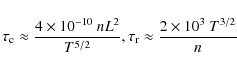 |
(1) |
(here, and in what follows, in all practical formulae the units of
![\begin{figure}
\par\includegraphics[width=16cm]{fig02a.eps}
\end{figure}](/articles/aa/full_html/2009/19/aa11872-09/img19.png) |
Figure 2: Scatter plots for mean intensity detected by TRACE and SXT. Dashed lines exhibit apparent lower limits of the TRACE intensity (Sakamoto 2006). |
| Open with DEXTER | |
Therefore, at any instant there are on average,
![]() filaments inside the loop that are
visible by TRACE, of which
filaments inside the loop that are
visible by TRACE, of which
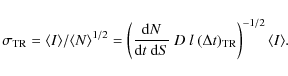
![]() (see Fig. 1) contribute to the intensity detected by a single pixel of
projection size l. Then, the mean emission count of the TRACE pixel can be calculated as
(see Fig. 1) contribute to the intensity detected by a single pixel of
projection size l. Then, the mean emission count of the TRACE pixel can be calculated as
| (2) |
where
 |
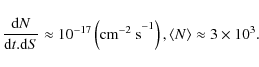
(3) |
The TRACE observations considered by Sakamoto et al. (2008) yield a wide range of emission counts for different pixels, for which more significant intensity fluctuations are found in brighter pixels. In this case, the following relation between
| (4) |
Furthermore, the auto-correlation time for the TRACE light curve was also derived (see Fig. 9 of Sakamoto et al. 2008) as
| (5) |
Finally, TRACE images of the entire active region allows one to estimate the ``averaged'' half-length and diameter of the loop as
 |
(6) |
We now consider other parameters of a TRACE filament with
We note that the aforementioned estimate for
![]() is an order of magnitude higher than the one predicted by the Rosner-Tucker-Vaiana (RTV) scaling (Rosner et al. 1978):
is an order of magnitude higher than the one predicted by the Rosner-Tucker-Vaiana (RTV) scaling (Rosner et al. 1978):
| (7) |
which yields the density
2.2 Implications for nanoflares
This interpretation of the TRACE-detected filaments presumes that they appear as a result of cooling of initially hotter and denser filaments, which
dominate the coronal differential emission measure and, hence, control the overall coronal energy budget. It is, therefore, important to deduce
their parameters from the theoretical modelling of nanoflare heating, and then to compare the findings with available simultaneous observations with
Yohkoh/SXT. Unlike TRACE, the SXT is a broad-band instrument ensuring that it is well-suited to probing this part of the coronal differential emission
measure. Clearly, if the nanoflare scenario of coronal heating does take place, one might expect a strong correlation between the emission intensities
detected by these two instruments, and this is exactly what is revealed by observations. Thus, Fig. 2 displays scatter plots for mean intensity detected by
TRACE and Yohkoh/SXT, where each dot corresponds to a pixel of the observed image (note that TRACE ![]() macropixels used here have almost the
same resolution as Yohkoh/SXT pixels).
The distribution shown in Fig. 2a, which corresponds to solar disk, is dominated by pixels bright in TRACE and dim in SXT. This is because of the
contribution of moss regions (Berger et al. 1999), which are footpoints of hot coronal loops heated by heat flux from the upper corona (Katsukawa &
Tsuneta 2005). Therefore, they do not represent coronal filaments produced by nanoflares and, hence, were excluded from the analysis of Sakamoto
et al. (2008). On the other hand, Fig. 2b, which corresponds to the solar limb, seems to be free of them, and it indeed exhibits the sought-after
correlation. Thus, for the aforementioned bright TRACE pixels with the mean emission count
macropixels used here have almost the
same resolution as Yohkoh/SXT pixels).
The distribution shown in Fig. 2a, which corresponds to solar disk, is dominated by pixels bright in TRACE and dim in SXT. This is because of the
contribution of moss regions (Berger et al. 1999), which are footpoints of hot coronal loops heated by heat flux from the upper corona (Katsukawa &
Tsuneta 2005). Therefore, they do not represent coronal filaments produced by nanoflares and, hence, were excluded from the analysis of Sakamoto
et al. (2008). On the other hand, Fig. 2b, which corresponds to the solar limb, seems to be free of them, and it indeed exhibits the sought-after
correlation. Thus, for the aforementioned bright TRACE pixels with the mean emission count
![]() taken with the exposure time
taken with the exposure time
![]() ,
the respective TRACE intensity of Fig. 2b equals
,
the respective TRACE intensity of Fig. 2b equals
![]() .
According to
Fig. 2b, it then corresponds to the SXT intensity
.
According to
Fig. 2b, it then corresponds to the SXT intensity
![]() ,
which for the SXT exposure time
,
which for the SXT exposure time
![]() yields the mean pixel emission count
yields the mean pixel emission count
![]() .
.
We now compare this number with theoretical predictions. It has been demonstrated (Cargill 1994; Vekstein & Katsukawa 2000)
that the maximum of the differential emission measure is provided by filaments that are in transition from the conductive to the radiation cooling stages, so that their conductive and radiation cooling times given by Eq. (1) are equal. This means that despite the impulsive nature of the nanoflare heating,
the temperature of these filaments, T*, and their density, n*, obey the RTV scaling of Eq. (7) that was originally derived for a state of static
thermal equilibrium. Furthermore, because of a broad temperature response function of SXT, the coronal loop temperature obtained with this instrument is
close to T*. Hence, the observed SXT temperature
![]() yields, according to the RTV scaling (7), the density
yields, according to the RTV scaling (7), the density
![]() .
As seen, the drop in the filament temperature,
.
As seen, the drop in the filament temperature,
![]() ,
by a factor of 5 results in a density
reduction,
,
by a factor of 5 results in a density
reduction,
![]() ,
of a factor of only 1.75, i.e., during the radiation cooling, the scaling
,
of a factor of only 1.75, i.e., during the radiation cooling, the scaling
![]() holds. This rate of material leaving the radiatively cooling filament is close to the value predicted by numerical simulations (Jakimiec et al. 1992; Cargill et al. 1995). At this temperature and density the lifetime of SXT-detected filaments is, according to Eq. (1), equal to
holds. This rate of material leaving the radiatively cooling filament is close to the value predicted by numerical simulations (Jakimiec et al. 1992; Cargill et al. 1995). At this temperature and density the lifetime of SXT-detected filaments is, according to Eq. (1), equal to
![]() ,
which is six times longer than
,
which is six times longer than
![]() .
This implies that hot, dense filaments observed by SXT have
filling factors as large as
.
This implies that hot, dense filaments observed by SXT have
filling factors as large as
![]() in the bright area of the coronal active region. The same trend of higher filling factors being detected by broad-band instruments, was also reported for simultaneous NIXT and Yohkoh/SXT data presented by Di Matteo et al. (1999). The respective SXT mean emission count
per pixel can be derived to be (see Fig. 1):
in the bright area of the coronal active region. The same trend of higher filling factors being detected by broad-band instruments, was also reported for simultaneous NIXT and Yohkoh/SXT data presented by Di Matteo et al. (1999). The respective SXT mean emission count
per pixel can be derived to be (see Fig. 1):
![]() ,
which as an
estimate
is quite consistent with the one evaluated above from Fig. 2b, where
,
which as an
estimate
is quite consistent with the one evaluated above from Fig. 2b, where
![]() is the response coefficient for the Al.1 filter of SXT (Tsuneta et al. 1991).
is the response coefficient for the Al.1 filter of SXT (Tsuneta et al. 1991).
Furthermore, during the conductive stage of cooling the total thermal energy of the filament does not change because the decrease in the plasma
temperature is compensated by the increase in its density due to chromospheric evaporation (Cargill 1994). Therefore, thermal energy of SXT filaments
is indicative of the initial energy input, i.e., the energy of nanoflares. This yields the following estimate for the nanoflare energy:
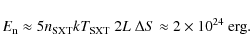 |
(8) |
Consequently, the overall energy budget in the active region area covered by bright pixels becomes equal to
 |
(9) |
3 Summary and conclusions
We have demonstrated that the analysis of small fluctuations in the coronal emission can provide an effective tool for probing the mechanism that maintains high plasma temperature in the corona of the Sun. The presented study highlights strongly the impulsive nature of the coronal heating by numerous energy-deposition events (nanoflares). It is shown how simultaneous TRACE and Yohkoh/SXT observations can be used for deducing the occurrence rate and the energy of individual nanoflares, as well as the overall energy budget of the coronal active region.
The suggested heating scenario, when the hot corona is viewed as a superposition of impulsively heated strands (filaments) provides a self-consistent interpretation of observational data and resolves some difficulties met by the static heating models (such as, for example, ``over-density'' of TRACE loops). It also implies that discussions (see, e.g. Aschwanden et al. 2007)about the true location of a primary energy release (e.g., upper chromosphere, or lower corona) are not so relevant because the subsequent chromospheric evaporation brings about the very same observable consequences.
Finally, this corona does not represent a steady heating of a pre-existing hot dense plasma: the primary magnetic energy dissipation is likely to occur in a much cooler and rarefied environment. This may have important implications for evaluating the effectiveness of various energy-release mechanisms, such as magnetic reconnection (see, e.g., Uzdensky 2007).
Acknowledgements
This work was supported by the United Kingdom STFC Research Council. The author is also grateful to Y. Sakamoto for the permission to reproduce Figs. 1 and 2, to S. Tsuneta for stimulating discussions, and to the anonymous referee for helpful comments.
References
- Aschwanden, M. J., Tarbell, T. D., Nightingale, R. W., et al. 2000, ApJ., 535, 1047 [NASA ADS] [CrossRef] (In the text)
- Aschwanden, M. J., Winebarger, A., Tsiklauri, D., et al. 2007, ApJ, 659, 1673 [NASA ADS] [CrossRef] (In the text)
- Benz, A. O., & Krucker, S. 2002, ApJ, 568, 413 [NASA ADS] [CrossRef] (In the text)
- Berger, T. E., de Pontieu, B., Schrijver, C. J., et al. 1999, ApJ, 519, L97 [NASA ADS] [CrossRef] (In the text)
- Cargill, P. J. 1994, ApJ, 422, 381 [NASA ADS] [CrossRef] (In the text)
- Cargill, P. J., Mariska, J. T., & Antiochos, S. K. 1995, ApJ, 439, 1034 [NASA ADS] [CrossRef] (In the text)
- Crosby, N. B., Aschwanden, M. J., & Dennis, B. R. 1993, Sol. Phys., 143, 275 [NASA ADS] [CrossRef] (In the text)
- Di Matteo, V., Reale, F., Peres, G., & Golub, L. 1999, A&A, 342, 563 [NASA ADS] (In the text)
- Drake, J. F. 1971, Sol. Phys., 16, 152 [NASA ADS] [CrossRef] (In the text)
- Handy, B. N., Acton, L. W., Kankelborg, C. C., et al. 1999, Sol. Phys., 187, 229 [NASA ADS] [CrossRef] (In the text)
- Hudson, H. S. 1991, Sol. Phys., 133, 357 [NASA ADS] [CrossRef] (In the text)
- Jakimiec, J., Sylwester, B., Sylwester, J., et al. 1992, A&A, 253, 269 [NASA ADS] (In the text)
- Katsukawa, Y. 2003, PASJ, 55, 1025 [NASA ADS] (In the text)
- Katsukawa, Y., & Tsuneta, S. 2001, ApJ, 557, 343 [NASA ADS] [CrossRef] (In the text)
- Katsukawa, Y., & Tsuneta, S. 2005, ApJ, 621, 498 [NASA ADS] [CrossRef] (In the text)
- Klimchuk, J. A. 2006, Sol. Phys., 234, 41 [NASA ADS] [CrossRef] (In the text)
- Krucker, S., & Benz, A. O. 1998, ApJ, 501, L213 [NASA ADS] [CrossRef] (In the text)
- Lin, R. P., Schwartz, R. A., Kane, S. R., Pelling, R. M., & Hurley, K. C. 1984, ApJ, 283, 421 [NASA ADS] [CrossRef] (In the text)
- Low, B. C., & Wolfson, R. 1988, ApJ, 324, 574 [NASA ADS] [CrossRef] (In the text)
- Parnell, C. E., & Jupp, P. E. 2000, ApJ, 529, 554 [NASA ADS] [CrossRef] (In the text)
- Parker, E. N. 1972, ApJ, 174, 499 [NASA ADS] [CrossRef] (In the text)
- Parker, E. N. 1988, ApJ, 330, 474 [NASA ADS] [CrossRef] (In the text)
- Rosner, R., Tucker, W. H., & Vaiana, G. S. 1978, ApJ, 220, 643 [NASA ADS] [CrossRef] (In the text)
- Sakamoto, Y. 2006, Ph.D. Thesis, University of Tokyo (In the text)
- Sakamoto, Y., Tsuneta, S., & Vekstein, G. 2008, ApJ, 689, 1421 [NASA ADS] [CrossRef] (In the text)
- Shimizu, T. 1995, PASJ, 47, 251 [NASA ADS] (In the text)
- Shimizu, T., & Tsuneta, S. 1997, ApJ, 486, 1045 [NASA ADS] [CrossRef] (In the text)
- Tsuneta, S., Acton, L., Bruner, M., et al. 1991, Sol. Phys., 136, 37 [NASA ADS] [CrossRef] (In the text)
- Uzdensky, D. A. 2007, ApJ, 671, 2139 [NASA ADS] [CrossRef] (In the text)
- Vekstein, G., & Katsukawa, Y. 2000, ApJ, 541, 1096 [NASA ADS] [CrossRef] (In the text)
- Vekstein, G., & Jain, R. 2003, Plasma Phys. Contr. Fusion, 45, 535 [NASA ADS] [CrossRef] (In the text)
- Vekstein, G., Priest, E. R., & Amari, T. 1991, A&A, 243, 492 [NASA ADS] (In the text)
- Wineberger, A. R., Warren, H. P., & Mariska, J. T. 2003, ApJ, 587, 439 [NASA ADS] [CrossRef] (In the text)
All Figures
| |
Figure 1: Schematic diagram of a coronal-loop observation (Sakamoto et al. 2008). |
| Open with DEXTER | |
| In the text | |
| |
Figure 2: Scatter plots for mean intensity detected by TRACE and SXT. Dashed lines exhibit apparent lower limits of the TRACE intensity (Sakamoto 2006). |
| Open with DEXTER | |
| In the text | |
Copyright ESO 2009
Current usage metrics show cumulative count of Article Views (full-text article views including HTML views, PDF and ePub downloads, according to the available data) and Abstracts Views on Vision4Press platform.
Data correspond to usage on the plateform after 2015. The current usage metrics is available 48-96 hours after online publication and is updated daily on week days.
Initial download of the metrics may take a while.