| Issue |
A&A
Volume 519, September 2010
|
|
|---|---|---|
| Article Number | A43 | |
| Number of page(s) | 5 | |
| Section | The Sun | |
| DOI | https://doi.org/10.1051/0004-6361/201014504 | |
| Published online | 09 September 2010 | |
Application of the theory of damping of kink oscillations by radiative cooling of coronal loop plasma
R. J. Morton - R. Erdélyi
Solar Physics and Space Plasma Research Centre (SP2RC), University of Sheffield, Hicks Building, Hounsfield Road, Sheffield S3 7RH, UK
Received 25 March 2010 / Accepted 18 May 2010
Abstract
Aims. We present here a first comparative study between the
observed damping of numerous fast kink oscillations and the theoretical
model of their damping due to the cooling of coronal loops. The theory
of damping of kink oscillations due to radiation of the solar plasma
with a temporally varying background is applied here to all known cases
of coronal kink oscillations.
Methods. A recent dynamic model of cooling coronal loops
predicts that transverse oscillations of such loops could be
significantly damped due to the radiative cooling process (Morton & Erdélyi 2009,
ApJ, 707, 750). The cooling of the loop plasma also has the consequence
that the kink oscillation has a time-dependent frequency. The theory is
applied to a relatively large number of known and reported examples of
TRACE observations of damped kink oscillations.
Results. We find that, for cooling timescales that are typical of EUV loops (
500-2000 s), the observed damping of the transversal (i.e. kink)
oscillations can be accounted for almost entirely by the cooling
process in half of the examples. No other dissipative mechanism(s)
seems to be needed to model the damping. In the remaining other
examples, the cooling process does not appear to be able to account
fully for the observed damping, though could still have a significant
influence on the damping. In these cases another mechanism(s), e.g.
resonant absorption, may be additionally required to account for the
complete decay of oscillations. Also, we show that because of the
dynamic nature of the background plasma, allowing for a time-dependent
frequency provides a better fit profile for the data points of
observations than a fit profile with a constant frequency, opening
novel avenues for solar magneto-seismology.
Key words: magnetohydrodynamics (MHD) - plasmas - Sun: corona - waves
1 Introduction
The first spatially resolved oscillations in coronal loops where reported with the Transitional Region And Coronal Explorer (TRACE) satellite (e.g. Aschwanden et al. 1999). Due to the transverse nature of these oscillations, they where identified as the fast kink body magnetohydrodynamic (MHD) mode (Nakariakov et al. 1999). Since then, there have been a relatively large number of observations of kink oscillations making them a useful tool for diagnostics of the coronal plasma (see e.g. Andries et al. 2009; and Ruderman & Erdélyi 2009, for the most recent reviews on kink waves). One outstanding problem associated with the kink oscillations is that they are observed to be heavily damped, usually within 4-5 periods. The cause of the damping is, to date, still unknown. Resonant absorption is thought to be a strong candidate (Ruderman & Roberts 2002; Goossens et al. 2002) and in certain cases may provide an explanation for the observed damping (Arregui et al. 2007; Goossens et al. 2008). A working alternative is shown here.
In general, models of coronal loops that support MHD oscillations have been assumed to be static with respect to the background plasma quantities. However, the solar corona is known to be of a highly dynamic nature. One such dynamic feature which is ubiquitous and dominant in the corona and has been observed on numerous occasions is the cooling of coronal loops (e.g. López Fuentes et al. 2007; Aschwanden & Terradas 2008).
It was preferentially thought, up until fairly recently, that
coronal loops existed in a state close to that of static
equilibrium, where the heating balanced the cooling of the plasma.
However, the static equilibrium models could not reproduce the
observed properties of large EUV coronal loops
(Aschwanden et al. 2000a). On the other hand, thermal non-equilibrium
models are found to be able to account for many observed properties
(see, e.g. Klimchuk et al. 2009). These models suggest that coronal
loops undergo cycles of heating and cooling phases over their
lifetimes, with the heating phase being rapid compared to the slow
cooling phase. This process has been observed on numerous occasions. One such typical example
is coronal loops being heated to soft X-ray temperatures, T> 2 MK,
before cooling down through to the EUV temperature range,
![]() MK (Nagata et al. 2003; Winebarger & Warren 2005;
Taroyan et al. 2007). Further, Reale et al. (2000) reported the
complete heating and cooling of a loop within the EUV temperature range.
MK (Nagata et al. 2003; Winebarger & Warren 2005;
Taroyan et al. 2007). Further, Reale et al. (2000) reported the
complete heating and cooling of a loop within the EUV temperature range.
Loops can also experience a localised heating, e.g. due to flares, which are also the suggested drivers for EUV kink oscillations. Simulations by Jakimiec et al. (1992) of flaring loops show the loops experience an initial, short lived heating phase followed by a slow cooling phase. There is mounting observational evidence for this phenomena. Ofman & Wang (2008) and Erdélyi & Taroyan (2008) both observed separate flaring events taking place in the vicinity of loop footpoints. The heating and cooling phases where identified in both observations and transverse oscillations in the loops where also reported.
Cooling timescales for EUV loops have been estimated in Aschwanden & Terradas (2008) to be around 500-2000 s. These cooling timescales are mostly larger though sometimes comparable to the characteristic timescale of the transverse oscillations, e.g. for fast kink body modes the oscillations have typical periods of 300-500 s and last for four to five periods, so the cooling of the loops is expected to influence the oscillations and the use of static background in the modelling of coronal loops is not necessarily justified (Aschwanden & Terradas 2008).
A new theoretical model of oscillating cooling coronal loops is developed by Morton & Erdélyi (2009, ME09 hereafter) who suggest that as a coronal loop cools, transverse MHD oscillations of the loops are considerably damped by the cooling of the plasma (see, ME09 for full details on the theoretical model and assumptions made). Here we put the theory outlined by ME09 to a rigorous test by applying it to 27 known examples of damped kink oscillations observed with TRACE and compare the observed rate of damping with the theoretically predicted damping due the cooling of the loop. Next, we also progress by proposing to investigate the time-dependent nature of oscillatory frequencies, opening new avenues in solar magneto-seismology. Often in reports of coronal loop oscillations it is very hard to distinguish between various modes of oscillations (i.e. fundamental, first harmonic, etc.) being present in the system as the mode periods evolve during the observations. Such time dependent periods are found in wavelet analysis (e.g. De Moortel et al. 2004). Strong dynamical behavior in the system could lead to the misinterpretation of data as showing many harmonics when in fact it is just one mode experiencing a change in period.
2 Key points of theory
Here we only recall very briefly the key points and results of the theory describing kink oscillations in a cooling coronal loop developed by ME09 that are essential to test the theory. The loop is considered to be longitudinally stratified with a semi-circular geometry in a gravitationally stratified atmosphere. The temperature of the loop is assumed to be isothermal and to evolve over time with an exponential profile. These assumptions serve as a good working approximation of the observed cooling of loops (Aschwanden & Terradas 2008; Ugarte-Urra et al. 2009), where the important new physics is still captured. A microphysical process of cooling (i.e. thermal conduction or radiation) is ignored and the effect of cooling on the density profile of the loop is concentrated on. The solution to the equation of motion for MHD plasmas with a time dependent density profile requires that the loop has a background flow. This dynamic background profile of the loop causes the loop to be slowly evacuated as it cools and the plasma flows out of the loop at the footpoints. Note, this is a strongly non-conservative physical system.
![\begin{figure}
\par\includegraphics[width=18.5cm,clip]{14504fg1.eps}
\end{figure}](/articles/aa/full_html/2010/11/aa14504-10/img2.png)
|
Figure 1: Examples of typical kink oscillations damped by radiation. The crosses are the observed data points (Nakariakov et al. 1999) and Aschwanden et al. (2002), solid black line is the fitted sine function Eq. (4). The various dashed lines are the envelope damping profiles due to cooling. In the text the individual plots are referred to as such, from left to right, top to bottom, a, b,...f, respectively. |
| Open with DEXTER | |
The radial velocity component in
transversal oscillations in cylindrical geometry takes the form,
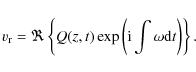
|
(1) |
Here Q(z,t) is the dynamic amplitude,
where
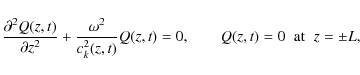
There are a number of interesting effects on the transverse oscillations
as the loop cools. Solutions to Eq. (2) show that as the
loop cools, transverse oscillations of the loop are damped due to
the cooling process. The rate of damping was also found to dependent
upon the initial temperature of the loop as the oscillation started,
the height of the loop apex in the atmosphere and the cooling
timescale,
![]() .
Another point that should be emphasised
and is important to applications of solar magneto-seismology is the
change in period of the modes. An analytic expression can be found
for the period change if a solution to Eq. (2) is sought
using the variational approach suggested by, e.g. McEwan et al. (2006).
Assuming that
.
Another point that should be emphasised
and is important to applications of solar magneto-seismology is the
change in period of the modes. An analytic expression can be found
for the period change if a solution to Eq. (2) is sought
using the variational approach suggested by, e.g. McEwan et al. (2006).
Assuming that
![]() where
where ![]() is height of loop apex above
photosphere and H is the scale height, then it is obtained for the
fundamental mode
is height of loop apex above
photosphere and H is the scale height, then it is obtained for the
fundamental mode
![\begin{displaymath}
P_1\approx
\frac{1}{c_{\rm kf}}{\frac{4L}{\pi^{3/2}}\left[{\...
...ght] \left(1+\delta \frac{t}{P}\right)}\right]^{\frac{1}{2}}},
\end{displaymath}](/articles/aa/full_html/2010/11/aa14504-10/img13.png)
where
3 Application to observed kink oscillations
Here we apply the theory to the 27 known damped kink oscillations
available in the current literature. In Fig. 1, we show
selected typical observations that have been identified as damped
fast kink oscillations, each of them observed by the TRACE
satellite. A catalogue of these observations is available in
Nakariakov et al. (1999) and Aschwanden et al. (2002). In order to apply the
theory, relevant information on the oscillations and their damping
characteristics is given in Table 1. The data points from
the observations have been fitted initially with a damped sine
function of the form
where
The damped oscillating coronal loops all appeared in the TRACE EUV
filters, either in the 171 Å or the 195 Å filter. The
filters have a broad temperature response where the 171 Å
filter has a peak response at
![]() MK and the 195 Å
at
MK and the 195 Å
at
![]() MK (Aschwanden et al. 2000b). This suggests that
the loop enters the 195 Å filter at a temperature of around
1.5 MK, so we set the initial temperature of the loop to about
1.5 MK as the oscillation begins and model a number of cooling
timescales that are representative of EUV loops, i.e.
500-2000 s.
The height of the loop apex is also required to determine the
fundamental period (see Eq. (3)) and is given in
Table 1. The damping profile is obtained by calculating the
value of
MK (Aschwanden et al. 2000b). This suggests that
the loop enters the 195 Å filter at a temperature of around
1.5 MK, so we set the initial temperature of the loop to about
1.5 MK as the oscillation begins and model a number of cooling
timescales that are representative of EUV loops, i.e.
500-2000 s.
The height of the loop apex is also required to determine the
fundamental period (see Eq. (3)) and is given in
Table 1. The damping profile is obtained by calculating the
value of ![]() at the loop apex, i.e. the maximum value of velocity
for the fundamental mode, and normalising with respect to the
initial value of
at the loop apex, i.e. the maximum value of velocity
for the fundamental mode, and normalising with respect to the
initial value of
![]() ,
i.e. the value at t=0. The normalised
damping profile is then scaled by the initial amplitude determined
from the fitted analytical function, Eq. (4), for each
oscillation and overplotted.
,
i.e. the value at t=0. The normalised
damping profile is then scaled by the initial amplitude determined
from the fitted analytical function, Eq. (4), for each
oscillation and overplotted.
Table 1: Information about oscillating loops shown in Fig. 1.
Most typical quoted examples in Fig. 1 show that the damping due to cooling (i.e. temporally varying background) is more than able to account for a significant amount of the observed decrease in amplitude. Analysing Fig. 1 suggests that the variable background (i.e. cooling of the plasma) offers a natural explanation for the damping of kink oscillations. In general, the degree of the match between theoretically predicted damping of the amplitudes of the oscillations and those detected by TRACE varies, depending upon the loop parameters. However, we find that in all cases, that we investigated, the dynamic background has at least some level of relevance for the damping. In Fig. 1a it can be seen that the theoretically predicted dynamic envelope profile of the damping due to cooling coincides very closely with that of the heuristically static fitted damping and is the best fit of all presented cases. The envelope from the damping due to cooling in Fig. 1b does not fit very closely the original damped sinusoidal profile by Aschwanden et al. (2002) but does include a number of the data points that are missed by this original profile. We then offer the view that the damping profile due to cooling can provide a better fit to the observed data points than the original heuristic fitted damping profile.
![\begin{figure}
\par\mbox{\includegraphics[width=8cm,clip]{14504fg2.eps}\hspace{0.5cm}
\includegraphics[width=8cm,clip]{14504fg3.eps} }\end{figure}](/articles/aa/full_html/2010/11/aa14504-10/img22.png)
|
Figure 2: In the left panel the oscillation in Fig. 1b is shown again here. Right panel shows Fig. 1e. Now plotted is the expected oscillation profile for the time dependent period substituted into the fitted sine function, Eq. (4). |
| Open with DEXTER | |
In Figs. 1c-e the
best fit damping profile from the cooling appears to be able to
match the heuristically static fitted damping profile less closely.
However, in Fig. 1c the cooling profile
provides a close fit for the oscillation from 1100 s. Anyway, in
all of these figures the best fit damping profile from the cooling
does however encompasses some of the data points that are outside
the envelope of the analytically fitted static damping profile. This
could be evidence that the originally fitted damping profile is not
the correct profile. Note that without error bars for the data, we
cannot rule out these outlying points could fall within the fitted
damping envelope. Unfortunately the error bars are not available in
their observational reports. A different explanation for the
difference between the best fit damping profile due to cooling and
the analytically fitted damping profile in
Figs. 1c-e can also
be offered. For each of these oscillations, note that the timescale
of the period, P, is close to that of the fitted damping time,
![]() ,
i.e. the damping is rapid compared to the period of the
oscillation. The reason that we have a disagreement between these
cooling and best fit damping profiles could be that the
characteristic cooling is less than 500 s. The practical
restriction placed upon the applicable allowed values of the ratio
,
i.e. the damping is rapid compared to the period of the
oscillation. The reason that we have a disagreement between these
cooling and best fit damping profiles could be that the
characteristic cooling is less than 500 s. The practical
restriction placed upon the applicable allowed values of the ratio
![]() by the WKB method, means that damping profiles
calculated for smaller values of
by the WKB method, means that damping profiles
calculated for smaller values of
![]() could have a
pronounced approximation error and we do not calculate the profiles
for less than 500 s here with the tools of the analytical theory.
For such cases a full numerical simulation would be required. An
alternative explanation for the discrepancy between the calculated
damping profiles and the observed profiles could be that another
dissipative process other than the cooling, e.g. resonant absorption,
has some important contribution to the damping of those particular
observations. Even so, it is clear that the cooling could still
provide a significant and dominant contribution to the damping for
these examples. In Fig. 1f it is suggestive that the best fit damping
profile from the cooling also does not fit well the observed damping
of the oscillation. The heuristically static fitted damping profile,
however, also does not fit a great number of the data points. This
leads to the suggestion that the oscillation may need to be
re-analysed or some existing physics is missing from the modelling.
could have a
pronounced approximation error and we do not calculate the profiles
for less than 500 s here with the tools of the analytical theory.
For such cases a full numerical simulation would be required. An
alternative explanation for the discrepancy between the calculated
damping profiles and the observed profiles could be that another
dissipative process other than the cooling, e.g. resonant absorption,
has some important contribution to the damping of those particular
observations. Even so, it is clear that the cooling could still
provide a significant and dominant contribution to the damping for
these examples. In Fig. 1f it is suggestive that the best fit damping
profile from the cooling also does not fit well the observed damping
of the oscillation. The heuristically static fitted damping profile,
however, also does not fit a great number of the data points. This
leads to the suggestion that the oscillation may need to be
re-analysed or some existing physics is missing from the modelling.
4 Issue on time-(in)dependent period
In the previous section it was pointed out while the loop cools the period
of the loop is also expected to change (see, e.g. Eq. (3)). In
the reported observations of the damped kink oscillations analysed
earlier by Nakariakov et al. (1999) and Aschwanden et al. (2002), the fitted
sine function has a constant period (time independent) and
apparently agrees with various degrees of success with the
observations. However, it should be noted the cadence for the TRACE
EUV imager is around 75 s, which will place a lower limit on the
periodicity that analysis will be able to determine from the
observations. Let us now re-analyse these loop oscillations assuming
that there is a variable background with allowed characteristic time
scales relevant to loop oscillations.
In the left panel of Fig. 2, applying the theory outlined in ME09,
we now plot the expected change in period if the loop is cooling
with a typical rate, say,
![]() s and starts
oscillating with the observed initial period 423 s. The estimated
damping time for this profile is the same as that for the original
static fitted profile. It can be seen that the revised
time-dependent quasi-sinusoidal profile fits the observations
equally as well if not better than the previous fit with constant
period. There is, however, a clearly identifiable
s and starts
oscillating with the observed initial period 423 s. The estimated
damping time for this profile is the same as that for the original
static fitted profile. It can be seen that the revised
time-dependent quasi-sinusoidal profile fits the observations
equally as well if not better than the previous fit with constant
period. There is, however, a clearly identifiable ![]()
![]() change
predicted in the period, where the period at the end of the
oscillation is around 100-120 s. A much improved cadence data is
now required to make further progress and confirm the period variations.
change
predicted in the period, where the period at the end of the
oscillation is around 100-120 s. A much improved cadence data is
now required to make further progress and confirm the period variations.
In the right panel of Fig. 2 we provide another typical
example. This time, however, we show the predicted period change for
a cooling timescale of
![]() s and we estimate the
fitted damping time so that it is also 700 s. Again, this allows
for a better fit between the observed data points and the
analytically fitted profile of the oscillation.
Comparing to Fig. 1e, it appears that the new fitted quasi-sinusoidal profile
of the analytically evolving loop oscillation, with changing period
and damping time of 700 s fits a greater number of the observed
data points than the one of a static kink oscillating coronal loop.
In both these examples the amplitude envelopes do not provide an
exact fit to the observed damping profile but the changing period
does provide a better fit for the data points. We suggest that it
may then be better to calculate the contribution of cooling to the
observed damping by first calculating the cooling time that
corresponds to the best fit period change. Fitting the corresponding
amplitude envelope for cooling will then show the contribution
needed by other mechanisms to account for the observed damping fully.
s and we estimate the
fitted damping time so that it is also 700 s. Again, this allows
for a better fit between the observed data points and the
analytically fitted profile of the oscillation.
Comparing to Fig. 1e, it appears that the new fitted quasi-sinusoidal profile
of the analytically evolving loop oscillation, with changing period
and damping time of 700 s fits a greater number of the observed
data points than the one of a static kink oscillating coronal loop.
In both these examples the amplitude envelopes do not provide an
exact fit to the observed damping profile but the changing period
does provide a better fit for the data points. We suggest that it
may then be better to calculate the contribution of cooling to the
observed damping by first calculating the cooling time that
corresponds to the best fit period change. Fitting the corresponding
amplitude envelope for cooling will then show the contribution
needed by other mechanisms to account for the observed damping fully.
In order to further support our dynamic modelling, it should be noted
that a ![]() decrease in period has already been tentatively
reported in De Moortel et al. (2004) who re-analysed the results from
Nakariakov et al. (1999). No explanation was provided for the decreasing
period in the study of De Moortel et al. (2004). The time dependent
background proposed here may offer the missing physics.
decrease in period has already been tentatively
reported in De Moortel et al. (2004) who re-analysed the results from
Nakariakov et al. (1999). No explanation was provided for the decreasing
period in the study of De Moortel et al. (2004). The time dependent
background proposed here may offer the missing physics.
5 Conclusions
We conclude that the damping due to a dynamic background could have
a dominant or at least significant influence on transverse
oscillations in EUV coronal loops. So far this theory seems to
describe best the observed features of damped kink oscillations and
concludes an important aspect of solar magneto-seismology. The
observed decay of these oscillations can be accurately predicted
only if the reported dynamic nature of the background plasma is also
adequately taken into account. The damping due to cooling (i.e.
variable background) seems to be a very plausible and natural
physical mechanism in most of the reported cases of kink
oscillations in loops. The variable background (i.e. time
dependent) certainly captures an important feature seen in many of
the oscillating post-flare coronal loops. This dissipative (and
non-conservative) physical process manages to explain the damping of
the loops without the need for an ansatz mechanism. Cooling occurs
ubiquitously in the corona and is expected to occur after a flaring
event in or close to the loop. The flare is a strong contender as
the driver for the transversal oscillation, so there will be a high
chance the loop is cooling while oscillating. In a number of the
currently known observed cases investigated, here we found that the
cooling can account almost entirely for the observed damping.
However, it appears another mechanism(s) of damping may still be
required so that the observed damping can be explained and
accurately modelled in some cases. We suggest to generalise
modelling efforts where both resonant absorption (i.e. the important
radial stratification) and a time dependent variable background are
both taken into account for oscillating coronal loops.
We also
suggest that a further observational signature of damping due to
cooling would be the decreasing period of the oscillation. Initial
evidence is provided in order to stimulate further investigation.
Allowing the period of the oscillation to change appears to be able
to match the observations better than static loop modelling
(although empirical error estimates of the measured amplitudes are
![]() - private communication M. Aschwanden). Whether we will be
able to detect the change in period with current cadences onboard
satellites will remain to be seen.
- private communication M. Aschwanden). Whether we will be
able to detect the change in period with current cadences onboard
satellites will remain to be seen.
R.E. acknowledges M. Kéray for patient encouragement. The authors are also grateful to NSF, Hungary (OTKA, Ref. No. K67746) and the Science and Technology Facilities Council (STFC), UK for the financial support they received.
References
- Andries, J., van Doorsselaere, T., Roberts, B., et al. 2009, Space Sci. Rev., 149, 3 [NASA ADS] [CrossRef] [Google Scholar]
- Arregui, I., Andries, J., Van Doorsselaere, T., Goossens, M., & Poedts, S. 2007, A&A, 463, 333 [NASA ADS] [CrossRef] [EDP Sciences] [Google Scholar]
- Aschwanden, M. J., & Terradas, J. 2008, ApJ, 686, L127 [NASA ADS] [CrossRef] [Google Scholar]
- Aschwanden, M. J., Fletcher, L., Schrijver, C. J., & Alexander, D. 1999, ApJ, 520, 880 [NASA ADS] [CrossRef] [Google Scholar]
- Aschwanden, M. J., Nightingale, R. W., & Alexander, D. 2000a, ApJ, 541, 1059 [NASA ADS] [CrossRef] [Google Scholar]
- Aschwanden, M. J., Tarbell, T. D., Nightingale, R. W., et al. 2000b, ApJ, 535, 1047 [NASA ADS] [CrossRef] [Google Scholar]
- Aschwanden, M. J., de Pontieu, B., Schrijver, C. J., & Title, A. M. 2002, Sol. Phys., 206, 99 [NASA ADS] [CrossRef] [Google Scholar]
- Bender, C. M., & Orszag, S. A. 1978, Advanced Mathematical Methods for Scientists and Engineers (New York: McGraw-Hill) [Google Scholar]
- De Moortel, I., Munday, S. A., & Hood, A. W. 2004, Sol. Phys., 222, 203 [NASA ADS] [CrossRef] [Google Scholar]
- Dymova, M. V., & Ruderman, M. S. 2005, Sol. Phys., 229, 79 [NASA ADS] [CrossRef] [Google Scholar]
- Erdélyi, R., & Taroyan, Y. 2008, A&A, 489, L49 [NASA ADS] [CrossRef] [EDP Sciences] [Google Scholar]
- Goossens, M., Andries, J., & Aschwanden, M. J. 2002, A&A, 394, L39 [NASA ADS] [CrossRef] [EDP Sciences] [Google Scholar]
- Goossens, M., Arregui, I., Ballester, J. L., & Wang, T. J. 2008, A&A, 484, 851 [NASA ADS] [CrossRef] [EDP Sciences] [Google Scholar]
- Jakimiec, J., Sylwester, B., Sylwester, J., et al. 1992, A&A, 253, 269 [NASA ADS] [Google Scholar]
- Klimchuk, J. A., Karpen, J. T., & Antiochos, S. K. 2010, ApJ, 714, 1239 [NASA ADS] [CrossRef] [Google Scholar]
- López Fuentes, M. C., Klimchuk, J. A., & Mandrini, C. H. 2007, ApJ, 657, 1127 [NASA ADS] [CrossRef] [Google Scholar]
- McEwan, M. P., Donnelly, G. R., Díaz, A. J., & Roberts, B. 2006, A&A, 460, 893 [NASA ADS] [CrossRef] [EDP Sciences] [Google Scholar]
- Morton, R. J., & Erdélyi, R. 2009, ApJ, 707, 750 [NASA ADS] [CrossRef] [Google Scholar]
- Nagata, S., Hara, H., Kano, R., et al. 2003, ApJ, 590, 1095 [NASA ADS] [CrossRef] [Google Scholar]
- Nakariakov, V. M., Ofman, L., Deluca, E. E., Roberts, B., & Davila, J. M. 1999, Science, 285, 862 [NASA ADS] [CrossRef] [PubMed] [Google Scholar]
- Ofman, L., & Wang, T. J. 2008, A&A, 482, L9 [NASA ADS] [CrossRef] [EDP Sciences] [Google Scholar]
- Reale, F., Peres, G., Serio, S., DeLuca, E. E., & Golub, L. 2000, ApJ, 535, 412 [NASA ADS] [CrossRef] [Google Scholar]
- Ruderman, M. S., & Roberts, B. 2002, ApJ, 577, 475 [NASA ADS] [CrossRef] [Google Scholar]
- Ruderman, M. S., & Erdélyi, R. 2009, Space Sci. Rev., 149, 199 [NASA ADS] [CrossRef] [Google Scholar]
- Taroyan, Y., Erdélyi, R., Wang, T. J., & Bradshaw, S. J. 2007, ApJ, 659, L173 [NASA ADS] [CrossRef] [Google Scholar]
- Ugarte-Urra, I., Warren, H. P., & Brooks, D. H. 2009, ApJ, 695, 642 [NASA ADS] [CrossRef] [Google Scholar]
- Verth, G., & Erdélyi, R. 2008, A&A, 486, 1015 [NASA ADS] [CrossRef] [EDP Sciences] [Google Scholar]
- Winebarger, A. R., & Warren, H. P. 2005, ApJ, 626, 543 [NASA ADS] [CrossRef] [Google Scholar]
All Tables
Table 1: Information about oscillating loops shown in Fig. 1.
All Figures
|
|
Figure 1: Examples of typical kink oscillations damped by radiation. The crosses are the observed data points (Nakariakov et al. 1999) and Aschwanden et al. (2002), solid black line is the fitted sine function Eq. (4). The various dashed lines are the envelope damping profiles due to cooling. In the text the individual plots are referred to as such, from left to right, top to bottom, a, b,...f, respectively. |
| Open with DEXTER | |
| In the text | |
|
|
Figure 2: In the left panel the oscillation in Fig. 1b is shown again here. Right panel shows Fig. 1e. Now plotted is the expected oscillation profile for the time dependent period substituted into the fitted sine function, Eq. (4). |
| Open with DEXTER | |
| In the text | |
Copyright ESO 2010
Current usage metrics show cumulative count of Article Views (full-text article views including HTML views, PDF and ePub downloads, according to the available data) and Abstracts Views on Vision4Press platform.
Data correspond to usage on the plateform after 2015. The current usage metrics is available 48-96 hours after online publication and is updated daily on week days.
Initial download of the metrics may take a while.