| Issue |
A&A
Volume 581, September 2015
|
|
|---|---|---|
| Article Number | A28 | |
| Number of page(s) | 30 | |
| Section | Stellar structure and evolution | |
| DOI | https://doi.org/10.1051/0004-6361/201526217 | |
| Published online | 27 August 2015 | |
Online material
Appendix A: Quality screening of the 2XMM light-curves
We list here the main features found in the data products that were likely to compromise the quality of the light-curves with respect to validity of the detection of “variability” and its characterisation. These features were identified mainly from visual inspection of the graphical products. Identification of any of these features in a dataset led to rejection of the light-curve for the present work.
Type of feature and number of 2XMM-Tycho variable detections rejected:
-
Optical loading (see 2XMM Appendix A): 11.
-
Confusion and contamination of source flux by another (usually brighter) nearby source: 8.
-
Problems in the background determination (e.g. poor background subtraction, background contamination from a nearby source): 7.
-
Exposure correction or GTI problem (leading to zeros or NULL-values in some of the source light-curve bins): 2.
-
Spurious detection (due to a nearby bright source): 1.
Thus in total, 29 out of the 157 2XMM-Tycho variable detections were rejected.
Of these 29, 11 had 2XMM SUM_FLAG ≥ 3, and none had SUM_FLAG=2 (see 2XMM Appendix D, Sect. D.5 for description of the SUM_FLAG values).
Appendix B: Calculation of the “completeness correction factor” C
Here we outline the calculation of the correction factor, C, used in Sect. 7.4.2 to account for variations in the minimum detectable flare strength. These arose mainly from the source quiescent flux upon which the flare was superimposed. C is the fraction of the survey time in which the flare could have been detected. We note that our primary aim was to demonstrate that our flare rates and related estimates were insensitive to incompleteness at the levels of accuracy needed for our analysis and warranted by the limited numbers in our samples, i.e. to estimate C to better than a factor ~2 and to utilise it at relatively modest correction values, i.e. 1 /C ≲ 2. We wished to generate an estimate of C in a simple and rapid manner, and based on quantities directly available from the 2XMM catalogue, rather than, for example, engaging in extensive simulations.
The minimum flare peak flux detectable above a signal-to-noise threshold of SNmin is: ![]() (B.1)where σf,cat is the EPIC total-band flux error in the 2XMM catalogue (i.e. column ep_8_flux_err), τon is the observation duration (“on-time”), τdur is the flare duration, and S:N is evaluated over the time interval τdur (Sect. 3.1).
(B.1)where σf,cat is the EPIC total-band flux error in the 2XMM catalogue (i.e. column ep_8_flux_err), τon is the observation duration (“on-time”), τdur is the flare duration, and S:N is evaluated over the time interval τdur (Sect. 3.1).
The assumption here is that σf,cat provides a reasonable representation of the error on the source time-series. Comparison of the EPIC total-band count-rate error with the count-rate error derived directly from the individual camera (pn, MOS1, MOS2) light-curves indicates that the latter can be a up to a factor ~2 greater than the former (especially for MOS1, MOS2)20. As discussed in Sect. 7.4.2, we have examined the effects of such errors in C on the resulting flare rates and distributions. We have also verified that using σf,cat, rather than an error estimate based on the quiescent count rate from the light-curve, results in ≲20% change in the error value.
Strictly, the value of τon is not precisely determined, since it varies between cameras (pn, MOS1, MOS2), and a flare (or other variability) could be flagged in any of the active cameras. Our solution for the present purpose was to use MOS1 on-time if available, else MOS2, else pn. This introduces an acceptably small “uncertainty” in τon, e.g. ≲30% variation in derived τon in ~80% of cases.
C is given by the normalised, cumulative distribution of observation on-times, i.e.:  (B.2)where n is the total number of observations in the sample being considered (and will, in general, include observations where no flares were detected), and the set of [fX,peak,SNmin,i,i = 1,n] is ordered by increasing value.
C can also be expressed in terms of flare peak luminosity or emitted energy, via:
 where d is the source distance.
Alternatively, C can be expressed in terms of maximum observable distance:  Example curves are shown in Fig. 24.
Appendix C: Additional tables and figures
Appendix C.1: The stars in the 2XMM-Tycho flare survey
Table C.1. The stars in the 2XMM-Tycho flare survey (1 row per XMM observation).
Appendix C.2: The flares in the 2XMM-Tycho flare survey
Table C.2. The flares and other time-variability events in the 2XMM-Tycho flare survey (1 row per event).
Appendix C.3: X-ray and ultraviolet light-curves
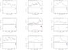 |
Fig. C.1
All 108 EPIC X-ray light-curves (top panel of each pair), and corresponding OM ultraviolet data (bottom panel of each pair) where available. Each pair of plots is labelled at the top with the 2XMM DETID, the star name, the EPIC camera and exposure number, and the X-ray time binning Δt (s). The conversion factor for count rates measured in the different EPIC cameras is 1 MOS count/s ≈ 3.2 PN count/s. The X-ray data are for the total energy band (0.2–12 keV); the OM waveband filters are indicated towards the right of the plot, and colour-coded. EPIC X-ray “flux” units are total-band count/s (in one of PN, MOS1, MOS2 cameras), while OM flux units are erg cm-2 s-1 Å-1 for imaging-mode data and count/s for fast-mode data. The conversion factors for OM count rates (count/s) to flux values are: 5.67 × 10⁻¹⁵ (W2), 2.20 × 10⁻¹⁵ (M2), 4.77 × 10⁻¹⁶ (W1), 1.99 × 10⁻¹⁶ (U), 1.24 × 10⁻¹⁶ (B), 2.51 × 10⁻¹⁶ (V) (XMM-SOC-CAL-TN-0019 http://xmm2.esac.esa.int/docs/documents/CAL-TN-0019.pdf Table 18.) The plots are ordered by 2XMM DETID; within each page, DETID increases from top to bottom, then right to left, starting at top right. |
| Open with DEXTER | |
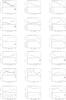 |
Fig. C.1
continued. |
| Open with DEXTER | |
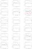 |
Fig. C.1
continued. |
| Open with DEXTER | |
Appendix C.4: X-ray count-rate and hardness-ratio light-curves
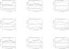 |
Fig. C.2
All 108 EPIC X-ray light-curves (top panel of each pair), and corresponding hardness-ratio light-curves with approximate temperatures indicated (bottom panel of each pair). Each pair of plots is labelled at the top with the 2XMM DETID, the star name, the EPIC camera and exposure number, and the X-ray time binning Δt (s). The conversion factor for count rates measured in the different EPIC cameras is 1 MOS count/s ≈ 3.2 PN count/s. The X-ray count rates are for the total energy band (0.2–12 keV), in one of PN, MOS1, MOS2 cameras. The hardness-ratios use bands 0.2–1, 1–12 keV. The plots are ordered by 2XMM DETID; within each page, DETID increases from top to bottom, then right to left, starting at top right. |
| Open with DEXTER | |
 |
Fig. C.2
continued. |
| Open with DEXTER | |
 |
Fig. C.2
continued. |
| Open with DEXTER | |
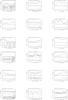 |
Fig. C.2
continued. |
| Open with DEXTER | |
 |
Fig. C.2
continued. |
| Open with DEXTER | |
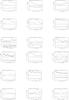 |
Fig. C.2
continued. |
| Open with DEXTER | |
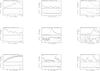 |
Fig. C.2
continued. |
| Open with DEXTER | |
© ESO, 2015
Current usage metrics show cumulative count of Article Views (full-text article views including HTML views, PDF and ePub downloads, according to the available data) and Abstracts Views on Vision4Press platform.
Data correspond to usage on the plateform after 2015. The current usage metrics is available 48-96 hours after online publication and is updated daily on week days.
Initial download of the metrics may take a while.