| Issue |
A&A
Volume 579, July 2015
|
|
|---|---|---|
| Article Number | A105 | |
| Number of page(s) | 19 | |
| Section | Interstellar and circumstellar matter | |
| DOI | https://doi.org/10.1051/0004-6361/201526117 | |
| Published online | 08 July 2015 | |
Online material
Appendix A: Gap depth − complete overview charts
The full overview charts for all molecules considered in our study are summarized in Fig. A.1 for the T Tauri case and in Fig. A.1 for the Herbig Ae case. The derived σ-weighted gap depth is color coded for each considered disk configuration.
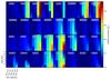 |
Fig. A.1
Overview plot of gap depth in the ideal velocity-channel maps for five different molecules. The central radiation source is a T Tauri star. The σ-weighted gap depth is color coded. |
| Open with DEXTER | |
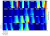 |
Fig. A.2
Overview plot of gap depth in the ideal velocity-channel maps for five different molecules. The central radiation source is a Herbig Ae star. The σ-weighted gap depth is color coded. |
| Open with DEXTER | |
Appendix B: Mol3D
In this section we present a detailed derivation of the underlying methods, physics, and assumptions used by our new N-LTE line and dust continuum radiative transfer code Mol3D.
Appendix B.1: Radiative transfer equations
We start with the transfer equation in the following form, ![]() (B.1)with the monochromatic intensity Iν, the emission factor jν(s), and the total absorption factor αν(s). The intensity from point p1 to p2 along its path s can be calculated using the integral form of Eq. (B.1),
(B.1)with the monochromatic intensity Iν, the emission factor jν(s), and the total absorption factor αν(s). The intensity from point p1 to p2 along its path s can be calculated using the integral form of Eq. (B.1), 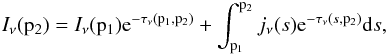 (B.2)where τν is the optical depth between two points, p1 and p2, along the ray of sight defined as
 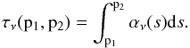 (B.3)
(B.3)
Appendix B.2: The gas-phase
For the gas, e.g., for a selected transition from lower level i to upper level j, the emission (jν) and absorption (αν) coefficients have the following form: 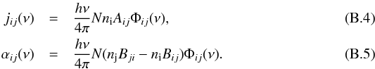 We follow the ansatz of Rybicki & Hummer (1991) for the non-overlapping multi-level line treatment. For a molecule with N levels and a selected transition between lower i and upper j level, we consider the spontaneous downward transition rates Aij, the Einstein coefficients Bij for stimulated transition, and the collision rate Cij. The collision rate can be calculated from the number density of the collision partner and the downward collision rate coefficient γij, which is the Maxwellian average of the collision cross section σ measured in laboratory:
 ![]() (B.6)All molecule data we use in our software package (e.g., frequencies, transition rates Aij, collision rate coefficients) are obtained from the Leiden Atomic and Molecular Database (LAMDA) (Schöier et al. 2005). As a consequence, Mol3D uses the same common input format for the molecule data as many other line radiative transfer programs available like RADEX (van der Tak et al. 2007) or URAN(IA) (Pavlyuchenkov & Shustov 2004). This approach offers the advantage of easily extending the code for several common molecules available in the LAMDA database (3 atomic and 33 molecular species at the time of writing). The dominant broadening effects are thermal and turbulent broadening. Hence, we assume a Gaussian line profile function, but in principle any other profile function can be included as well,
(B.6)All molecule data we use in our software package (e.g., frequencies, transition rates Aij, collision rate coefficients) are obtained from the Leiden Atomic and Molecular Database (LAMDA) (Schöier et al. 2005). As a consequence, Mol3D uses the same common input format for the molecule data as many other line radiative transfer programs available like RADEX (van der Tak et al. 2007) or URAN(IA) (Pavlyuchenkov & Shustov 2004). This approach offers the advantage of easily extending the code for several common molecules available in the LAMDA database (3 atomic and 33 molecular species at the time of writing). The dominant broadening effects are thermal and turbulent broadening. Hence, we assume a Gaussian line profile function, but in principle any other profile function can be included as well, 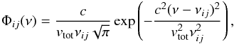 (B.7)where νij is the central frequency of the transition and c the speed of light. The parameter vtot gives the total line broadening factor taking into account the assumed microturbulent velocity vturb and the kinetic velocity vkin due to the kinetic temperature Tkin:
 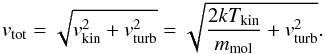 (B.8)In our code, the microturbulent velocity vturb can either be set to a common value, ~0.1−0.2 km s-1 for protoplanetary disks (Piétu et al. 2007; Hughes et al. 2011), or for example in the case of an outcome of (M)HD/MRI simulations, it can be provided as an input for every grid cell.
Finally, to describe the full line radiative transfer problem, a set of balance equations is needed: 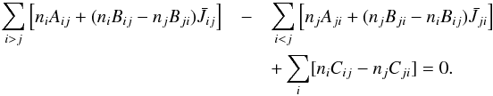 (B.9)In fact, Eq. (B.9) is not one single equation, but a whole set of linear equations, one for every energy level. In our code this linear matrix equation is solved with a simple Gaussian elimination algorithm. This set has to be solved locally (for every grid cell), but it has a global character due to its dependency on the line integrated mean intensity
 ![]() defined as
defined as  (B.10)Equations (B.9) and (B.10) are directly coupled to Eq. (B.1).
To solve the line radiative transfer problem, one needs to start with estimated values for the level populations, solve the radiative transfer equation, calculate the mean intensity, and then solve Eq. (B.9) again to create a new set of level populations. Then one needs to iterate until the correct level populations have been found.
Appendix B.2.1: Level populations
The main problem in radiative line transfer is the calculation of the level populations. Equation (B.9) shows that the level populations are directly coupled to the mean intensity and therefore to the gas temperature, which is unknown for complex structures as in the case of protoplanetary disks.
We implemented dissimilar algorithms to calculate the level populations with three approximate methods, for example, local thermodynamical equilibrium LTE, FEP, and LVG. As Pavlyuchenkov et al. (2007) have shown for the case of protoplanetary disks, for the most common molecules LVG is a very accurate method of calculating the level populations and gives a very good ratio between computational efficiency and reliability of the results.
LTE level populations
In this assumption the level populations follow a Boltzmann distribution and the excitation temperature of the selected transition is assumed to be equal to the kinetic temperature Texc = Tkin:  (B.11)Here gi and gj are the statistical weights of the i − j line transition and νij the corresponding central frequency.
LVG level populations
In the case of protoplanetary disks, the radial velocity gradients are usually much larger than the local thermal and microturbulent velocities (Weiß et al. 2005; Castro-Carrizo et al. 2007). This means that photons emitted at a certain disk region can only interact and consequently get absorbed locally. In this approach, the mean intensity J is approximated from the local source function S in combination with an external radiation field Jext:  The quantity β gives the probability of a photon beeing able to escaping the model. We note that in the optically thin case a photon can escape the model without interaction. For this case, β equals 1 and the LVG method would be equal to the full escape probability method. Therefore, the FEP method (also included in Mol3D) uses the same formalism as the LVG method, but with β always set to 1 (see also van der Tak et al. 2007). To calculate the local β, our program uses Eq. (B.14) introduced by Mihalas et al. (1978); de Jong et al. (1980) for accretion disks in general,
 ![]() (B.14)where τ is the effective optical depth of the observed line. We note that this formula is well suited in the case of proto-circumstellar disks. For other geometries and scenarios other approximations might give better results (see, e.g., de Jong et al. 1975 or Osterbrock & Ferland 2006). At this point an approximation of the optical line depth is made. As it is connected to the local velocity field V, microturbulence vturb, and gas density, we use the following expression (see also Pavlyuchenkov et al. 2007):
(B.14)where τ is the effective optical depth of the observed line. We note that this formula is well suited in the case of proto-circumstellar disks. For other geometries and scenarios other approximations might give better results (see, e.g., de Jong et al. 1975 or Osterbrock & Ferland 2006). At this point an approximation of the optical line depth is made. As it is connected to the local velocity field V, microturbulence vturb, and gas density, we use the following expression (see also Pavlyuchenkov et al. 2007):  (B.15)
Appendix B.3: Benchmarks
We demonstrate the applicability of the code Mol3D. For this purpose we compare its results to those obtained with the line radiative transfer code URAN(IA) (Pavlyuchenkov & Shustov 2004) and the dust continuum radiative transfer code MC3D (Wolf et al. 1999; Wolf 2003).
Appendix B.3.1: URAN(IA)
URAN(IA) is a 2D radiative transfer code for molecular lines. It features a Monte Carlo algorithm for calculating the mean intensity and an accelerated lambda iteration (ALI) method for self-consistent molecular excitation calculations. This code has been extensively tested in 1D and 2D, for example against the RATRAN code (Hogerheijde & van der Tak 2000). It successfully passed all tests formulated in the benchmark paper for N-LTE molecular radiative transfer by van Zadelhoff et al. (2002). It has been used in several applications, for example modeling the starless core L1544 (Pavlyuchenkov & Shustov 2004), and in dedicated parameter space studies of molecular line formation of molecular line formation of prestellar cores (Pavlyuchenkov et al. 2008).
In this code, several approximate methods of calculating the level populations are included. In a comprehensive study, Pavlyuchenkov et al. (2007) have shown the reliability of these methods in protoplanetary disk scenarios.
In Sect. 2 we introduced the different methods of calculating level populations implemented in Mol3D. In Fig. B.1 we present the spectrum of the HCO+ (4−3) transition of a typical protoplanetary disk (Mdisk = 0.07 M⊙), comparing the different methods assuming a uniform N(HCO+)/N(H) ratio of 1 × 10⁻⁸. For simplicity, we choose a flared disk model around a T Tauri star utilizing a temperature distribution with a gradient in radial and vertical direction and a power-law model for the density distribution adapted from Shakura & Sunyaev (1973):  (B.16)The disk is orientated face-on. We assume pure Keplerian rotation and neglect dust re-emission. All spectra are normalized to the maximum value of the LTE solution. To allow comparison, the resulting spectra obtained with the URAN(IA) code are also included.
URAN(IA) and Mol3D produce comparable HCO+ (4−3) spectra with differences of less than about 0.5%. The most realistic solution (black line) is obtained using the accelerated Monte Carlo (ART), to classify the approximation methods. As discussed in greater detail in Appendix B.2.1, the LTE method overestimates the net flux and the FEP method underestimates it. The fluxes in the line obtained with the LVG method are in between those obtained with the other methods and are closely comparable to the ART method. This result has also been found by Pavlyuchenkov et al. (2007) and we refer the interested reader to their study.
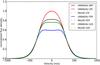 |
Fig. B.1
HCO+ (4−3) transition of a protoplanetary disk, oriented face-on. Different colors are obtained with different methods. Solid lines are obtained using the URAN(IA) software package and dotted lines represent solutions obtained with Mol3D. Shown is the normalized flux over velocity. Both codes produce comparable results within acceptable differences (less than 0.5%). LVG is a good approximation in the case of circumstellar disks (Pavlyuchenkov et al. 2007). |
| Open with DEXTER | |
Appendix B.3.2: MC3D
MC3D is a 3D continuum radiative transfer code that uses a Monte Carlo method to calculate self-consistent dust temperature distributions, continuum re-emission/scattering maps, and SEDs. Among a wide variety of radiative transfer studies it has been applied extensively for the analysis of multiwavelength high-angular-resolution observations of circumstellar disks (e.g., Schegerer et al. 2008; Sauter & Wolf 2011; Madlener et al. 2012; Gräfe & Wolf 2013). MC3D was successfully tested against other continuum RT codes (e.g., Pascucci et al. 2004).
In this section, we compare Mol3D with MC3D for a typical protoplanetary disk scenario. The density distribution is described by Eq. (B.16), assuming a total disk mass of 0.04 M⊙. The temperature structure is calculated self-consistently with
each code using their Monte Carlo scheme. Both codes use a similar approach based on the assumption of local thermal equilibrium and immediate temperature correction as proposed by Bjorkman & Wood (2001).
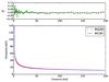 |
Fig. B.2
Midplane temperature of a typical protoplanetary disk around a pre-main-sequence T Tauri star. This disk inner radius amounts to 2 AU and the outer radius to 200 AU, respectively. The total disk mass amounts to 0.04 M⊙. Mol3D (red) and MC3D (blue) obtain comparable results. In this case, the differences depend significantly on the optical disk properties and subsequently on the number of photon packages simulated in the Monte Carlo process. Thus, the error is higher in the dense region at the inner rim of the disk (max. 10%) and lower at the outer disk regions (max. 2%). |
| Open with DEXTER | |
The resulting midplane temperature around a PMS T Tauri star is shown in Fig. B.2. The calculation of the temperature in the dense midplane is one of the most crucial RT problems, because these disk regions can hardly be reached by stellar photons directly. Thus, it is mostly heated indirectly by thermal re-emission radiation from the innermost disk regions and upper disk layers. Both codes produce very smooth and similar temperature distributions. The statistical nature of the Monte Carlo method results in deviations of about 10% for the innermost disk parts and less than 2% for the outer regions, which is mainly due to the probability that the photon packages can reach these regions.
We also compared the dust re-emission/scattered light maps and SEDs and find that both codes produce comparable results with maximum deviations of about 10%.
© ESO, 2015
Current usage metrics show cumulative count of Article Views (full-text article views including HTML views, PDF and ePub downloads, according to the available data) and Abstracts Views on Vision4Press platform.
Data correspond to usage on the plateform after 2015. The current usage metrics is available 48-96 hours after online publication and is updated daily on week days.
Initial download of the metrics may take a while.