| Issue |
A&A
Volume 579, July 2015
|
|
|---|---|---|
| Article Number | A59 | |
| Number of page(s) | 16 | |
| Section | Stellar structure and evolution | |
| DOI | https://doi.org/10.1051/0004-6361/201425568 | |
| Published online | 29 June 2015 | |
Online material
Appendix A: Synthetic dataset: sampling strategy
In constructing the sample adopted in the error estimation, we did not try to match any observed distribution of the mass of the binary stars or of the mass ratio q. Since we primarily aimed to investigate the performances of grid-based age estimates of binary stars, we paid more attention when sampling the whole range in mass, metallicity, and evolutionary phases covered by the available grid of models.
In detail, the datasets of artificial stars are sampled by adopting the following scheme. First, a star is randomly sampled from the grid. No priors on mass, age, and metallicity are assumed in the sampling procedure. Then, a second star is coupled to the first one with two requirements: it must share with the first star both the same initial [Fe/H] and the age, with a tolerance of 10 Myr. The couple of stars is re-ordered to have the most luminous star as a first member.
|
Fig. A.1
Left: joint density of mass and relative ages in the sample of primary stars. The colours correspond to the different densities of probability. Right: same as the left panel for secondary stars. The colour scales of the two panels are different. |
|
| Open with DEXTER | |
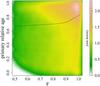 |
Fig. A.2
Joint density of mass ratio q and primary relative age in the sample of binary stars. The solid line displays the LOESS-smoothed trend of relative age versus mass ratio q. |
| Open with DEXTER | |
To show which models are selected as primary and secondary stars, we estimated the joint density of mass and relative age for primary and secondary stars9. From the joint density it is possible to verify if there are ranges of mass or relative age that are preferably sampled. The results are displayed in Fig. A.1. It is apparent that the density functions for the primary and secondary stars are different and that they are both not uniform. In particular, the sample of primary stars is biased towards high masses and high relative ages since these models have higher intrinsic luminosity. The distribution of secondary stars is more diffuse, since several young low-mass models are present in the sample. Figure A.2 shows the joint density of the mass ratio q and the primary relative age. The solid line in the figure is a LOESS smoother10 of the relative age versus q. It is apparent that for binary systems with near equal masses, the sampling returns more evolved stars. This bias comes from later evolutionary phases needing more points to adequately follow the rapid evolution. The median time step in this grid region is about 13 Myr. Once a model has been sampled in this grid region, several points in the same evolutionary track will pass the constraint on maximum age differences of 10 Myr from the first sampled model. Therefore there is a high probability that a point in the same track is coupled to the first selected stars, leading to a mass ratio of 1.0. This phenomenon is not important in the reconstruction phase, since all these points have basically the same age, as discussed in V15.
The effect of the sampling could be seen in Table 1, which shows a small shrink in the age relative error envelope at q greater than 0.9. This is a direct consequence of the relative error envelope narrowing at high relative age. To show that this artificial trend could be removed with different sampling strategies, in Table 1 we also present two additional series of results. In fact, we first explored the impact of a different sampling. For this test, we sampled the set of primary stars, then we coupled each of those objects to the secondary star by sampling only from the models respecting the constraint in metallicity and age, which are also less massive than the primary object. The results are in the rows labelled “mass ratio q (alternative sampling)” in Table 1. As a second test, to see the impact of the ad-hoc removal of the trend of primary relative ages versus q shown in Fig. A.2, we checked an alternative approach that rejects some objects in the subset q> 0.9, based on the standard method. In fact, since this is the region that is more populated, it was possible to draw from it a sample of size equal to that of the adjacent subset 0.8 <q ≤ 0.9, with the requirement that the new sample’s primary relative age matches the distribution of the subset 0.8 <q ≤ 0.9. The corresponding results are in the rows “mass
ratio q (rejection step)” in Table 1. It appears that the shrinkage in the upper q region is reduced in both two cases.
In contrast, the shrinkage of the error envelope at low mass ratio q (see Table 1) is due to an edge effect since there are only models in this region with mass 1.6 M⊙ coupled with 0.8 M⊙ models. In fact the lower left-hand region of Fig. A.2 is not populated because to produce a coeval combination, the more massive model cannot be too young. In fact, in this case the secondary is still in the pre-main sequence phase, which is not considered in the grid. Figure A.2 shows that the minimum relative age for these massive models is about 0.2. Therefore the most critical region for age estimation – that of low relative age – is avoided, and the estimate relative error envelope is narrower.
© ESO, 2015
Current usage metrics show cumulative count of Article Views (full-text article views including HTML views, PDF and ePub downloads, according to the available data) and Abstracts Views on Vision4Press platform.
Data correspond to usage on the plateform after 2015. The current usage metrics is available 48-96 hours after online publication and is updated daily on week days.
Initial download of the metrics may take a while.