| Issue |
A&A
Volume 576, April 2015
|
|
|---|---|---|
| Article Number | A84 | |
| Number of page(s) | 13 | |
| Section | Interstellar and circumstellar matter | |
| DOI | https://doi.org/10.1051/0004-6361/201424778 | |
| Published online | 02 April 2015 | |
Online material
Appendix A: Individual set of observations
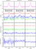 |
Fig. A.1
All three AMBER observations of HD 163296 with spectral resolution of 12 000. The three columns show the observed intereferometric results from 2012 May 11 (left), 2012 May 12 (middle), and 2012 June 04 (right). Shown from top to bottom are wavelength dependence of flux, visibilities, wavelength-differential phases (for better visibility, the differential phases of the first and last baselines are shifted by +50° and −50°, respectively), and closure phase observed at projected baselines as shown in the plot. The wavelength scale at the bottom is corrected to the local standard of rest. The typical visibilities, differential, and closure phases errors are ±5%, 5°, and 15°. |
| Open with DEXTER | |
Appendix B: Pure line visibilities
|
Fig. B.1
Comparison of the observed and modelled pure Brγ line visibilities of our AMBER observation of HD 163296. From top to bottom: wavelength dependence of flux, visibilities of the first, second, and third baseline. In each visibility panel: (1) the observed total visibilities (red, green, blue, as in Fig. 1); (2) the observed continuum-compensated pure Brγ line visibilities (pink), and the modelled pure Brγ line visibilities (black; model MW6, Table 3) are shown. |
|
| Open with DEXTER | |
Appendix C: Examples of computed disc wind models
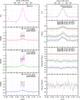 |
Fig. C.1
Same as Fig. B.1 (left panel) and Fig. 2 (right panel) but for model MW26 (see Table 3). |
| Open with DEXTER | |
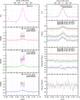 |
Fig. C.2
Same as Fig. B.1 (left panel) and Fig. 2 (right panel) but for model MW47 (see Table 3). |
| Open with DEXTER | |
Appendix D: Examples of computed hybrid models: disc wind plus magnetosphere
Appendix D.1: The magnestosphere
A full description of the model employed here can be found in Tambovtseva et al. (2014). Here, only a brief description of the main model parameters is presented.
Our model considers a compact, disc-like rotating magnetosphere of height hm through which free-falling gas reaches the stellar surface at some altitude near the magnetic pole. The gas rotational velocity component (u) is described by
![]() (D.1)where U0 is the rotational velocity of the gas at the magnetic poles, r is the distance from the star, and p is a parameter. Finally, we assume a dependence of the electron temperature (Te) of
(D.1)where U0 is the rotational velocity of the gas at the magnetic poles, r is the distance from the star, and p is a parameter. Finally, we assume a dependence of the electron temperature (Te) of ![]() (D.2)where r1 = ((r − R∗) /R∗)q, Te(R∗) is the temperature of the gas near the stellar surface, and q is a parameter.
(D.2)where r1 = ((r − R∗) /R∗)q, Te(R∗) is the temperature of the gas near the stellar surface, and q is a parameter.
Magnetosphere model parameters
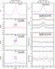 |
Fig. D.1
Same as Fig. B.1 (left panel) and Fig. 2 (right panel) but for the hybrid model MW6+MS6a (see Tables 3 and D.1). |
| Open with DEXTER | |
In our hybrid model, the magnetosphere is equivalent to a point source at our interferometer baselines. Thus, it accounts for the compact and unresolved Brγ emission, whereas the disc wind component is responsible of the resolved Brγ emission.
Because of the spread on the measured Ṁacc values, and the large uncertainties in measuring this quantity (~20%), an average value of 1 × 10⁻⁷ M⊙ yr-1 was assumed in our magnetosphere model.
© ESO, 2015
Current usage metrics show cumulative count of Article Views (full-text article views including HTML views, PDF and ePub downloads, according to the available data) and Abstracts Views on Vision4Press platform.
Data correspond to usage on the plateform after 2015. The current usage metrics is available 48-96 hours after online publication and is updated daily on week days.
Initial download of the metrics may take a while.