| Issue |
A&A
Volume 575, March 2015
|
|
|---|---|---|
| Article Number | A28 | |
| Number of page(s) | 17 | |
| Section | Planets and planetary systems | |
| DOI | https://doi.org/10.1051/0004-6361/201424964 | |
| Published online | 16 February 2015 | |
Online material
Appendix A: A simple model for evolving accretion discs
In this Appendix we provide a fit for our simulated disc models for all the different Ṁ stages. We provide here only a fit for the temperature T, because for discs with constant Ṁ, all other quantities can be derived, from the value of Ṁ and the α parameter. This is done by using the Ṁ relation and the hydrostatic equilibrium equation 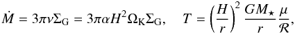 (A.1)where ℛ is the gas constant. The temperature given in the following fit is the mid-plane temperature of the disc, which does not represent the vertical structure of the disc that can feature a super-heated upper layer (e.g. Paper I). With the fit of the temperature, H can be determined and then finally ΣG.
We identify three different regimes for the temperature gradients in the disc. The inner disc is dominated by viscous heating and features a higher temperature than the water condensation temperature (Fig. A.1), while the outer disc is dominated by stellar irradiation. In between, the disc is in the shadow of stellar irradiation. This can be seen more clearly in the middle panel of Fig. 5, where H/r drops with increasing r. We fit each of these three regimes with individual power laws, which are indicated in Fig. A.1 as well.
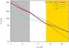 |
Fig. A.1
Radial temperature profile of the disc with Ṁ = 3.5 × 10⁻⁸ M⊙/yr. The different background colours mark different fit-regimes. The grey area marks the inner part of the disc that is dominated by viscous heating, while the golden part indicates the outer parts of the disc that is dominated by stellar heating. The white middle region indicates the shadowed region of the disc. |
| Open with DEXTER | |
The fit for the temperature for the outer part of the disc is T ∝ r− 4 / 7 which is steeper than in the MMSN and CY2010 models that are based on analytical arguments (e.g. Chiang & Goldreich 1997). The reason for this originates in the shadowed parts of the disc. The disc is cooler in the shadow and is heated by diffusion from the hotter inner part (heated viscously) and by the hotter outer part (heated from the star). This leads to a steeper temperature gradient in the outer parts, where the disc just emerges from the shadow, since it has to (partially) compensate for the lack of heating in the shadowed region. This compensation for heat influences the gradient in temperature to quite large distances. But we suspect that the gradient in temperature will return back to T ∝ r− 3 / 7 in the very outer parts of the disc, because the influence of the shadowed region reduces with larger orbital distances. This is also true for discs in the later stage evolution, since those discs no longer feature a prominent bump at the ice line that can shade parts of the disc from stellar irradiation.
The changes in the temperature gradient originate in the changes of opacity, which changes the cooling rate of the disc and hence the temperature (Paper II). The changes in opacity occur at the ice line, where ice grains melt and sublimate, and at the silicate line (≈1000 K). As Ṁ decreases, the viscous heating in the inner disc decreases as well, making the disc colder and moving the ice-line bump closer towards the central star. If the temperature of the disc is always below the water condensation temperature, the disc will therefore not feature the ice line bump any more (see Ṁ< 8.75 × 10⁻⁸ M⊙/yr in Fig. 5), and thus the inner part of the fit, which requires a higher temperature than the water condensation temperature, is not needed any more. Consequently, the fit of the temperature profile will only consist of fits of the middle and outer parts of the disc (indicated in white and yellow in Fig. A.1).
As long as the temperature is below the sublimation temperature of silicate grains (T< 1000 K), the fit can be applied to regions that are inside 1 AU. The reason for that is that there are no additional bumps in the opacity profile for 170 K <T< 1000 K that could change the disc structure by changing the cooling rate of the disc (Paper I).
As Ṁ decreases and the viscous heating in the inner parts of the disc decreases, the disc’s heating is dominated more and more by stellar irradiation. This transition in the dominant heating process occurs for Ṁ ≈ 1.75 × 10⁻⁸ M⊙/yr. We therefore observe a huge drop in the disc’s temperature (top panel in Figs. 5 and 8) around these Ṁ rates. For even lower Ṁ rates, the changes in temperature seem to be smaller again, which is caused by the fact that the disc’s heating is now entirely dominated by stellar irradiation. We therefore introduce different fitting regimes for different Ṁ values.
Since the heating and cooling of the disc is directly proportional to the Ṁ value, our fit is a function of Ṁ. We express each of the three individual power law fits in the following form ![]() (A.2)where A is a reference temperature expressed in K and B the factor by which the scaling with Ṁ is expressed through μR = log (Ṁ/Ṁref), where Ṁref is the reference Ṁ value. The factor ψij expresses the transition from regime i to regime j. The factor l corresponds to the power law index of the fit, shown in Fig. A.1.
(A.2)where A is a reference temperature expressed in K and B the factor by which the scaling with Ṁ is expressed through μR = log (Ṁ/Ṁref), where Ṁref is the reference Ṁ value. The factor ψij expresses the transition from regime i to regime j. The factor l corresponds to the power law index of the fit, shown in Fig. A.1.
In the inner regions of the disc for high Ṁ, the disc is dominated by viscous heating, and higher metallicity reduces the cooling, making the disc hotter, therefore increasing the temperature and the gradient of the temperature, which is then a function of metallicity. For Ṁ< 1.75 × 10⁻⁸ M⊙/yr, the disc starts to become dominated by stellar irradiation, so that the temperature gradient in the inner parts of the disc flattens. At the same Ṁ rates, the shadowed regions of the disc shrink, making the gradient of temperature in the outer parts of the disc flatter as well, because the outer parts of the disc no longer have to compensate for such a large unheated shadowed region.
The fit for the whole disc with Ṁ ≥ 1.75 × 10⁻⁸ M⊙/yr can therefore be expressed as 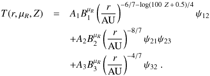 (A.3)For Ṁ< 1.75 × 10⁻⁸ M⊙/yr and Ṁ ≥ 8.75 × 10⁻⁹ M⊙/yr, the fit is expressed as
 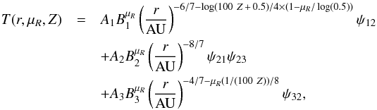 (A.4)where the gradient of the inner part of the disc relaxes back to r− 6 / 7 at Ṁ = 8.75 × 10⁻⁹ M⊙/yr, and the gradient of the outer part of the disc becomes less steep as a function of Z. For Ṁ< 8.75 × 10⁻⁹ M⊙/yr the fit is expressed as
 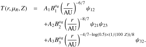 (A.5)These formula are used for both high and low metallicity discs.
The middle part contains two ψ functions since the second regime has to be smoothed into the first and into the third regime. For all different Ṁ fitting regimes the values of A, B, and ψ change, but keep the same shape.
Along with the changes in Ṁ, the disc changes as different metallicities provide different cooling rates and therefore different temperatures. These changes in temperature then reflect back on changes in H/r and ΣG. We therefore also introduce different regimes for the metallicity, where we distinguish between high metallicity (Z ≥ 0.005) and low metallicity (Z< 0.005). The factors A, B, and ψ are therefore functions of Ṁ and Z. The scaling with Z is expressed through χ = log (100Z/ 0.5) / log (2).
Appendix A.1: Low metallicity discs
In this section the fit for discs with Z< 0.005 is presented. The first regime of Ṁ is for Ṁ> 3.5 × 10⁻⁸ M⊙/yr, which corresponds to the early evolution of the disc. We define Ṁref = 3.5 × 10⁻⁸ M⊙/yr, and the fit reads as (where r is in units of AU) 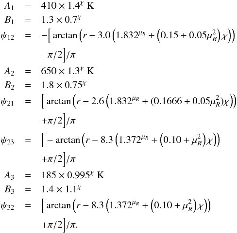 (A.6)The next regime spans the interval 1.75 × 10⁻⁸ M⊙/ yr <Ṁ ≤ 3.5 × 10⁻⁸ M⊙/yr and Ṁref = 3.5 × 10⁻⁸ M⊙/yr, and the fit reads as
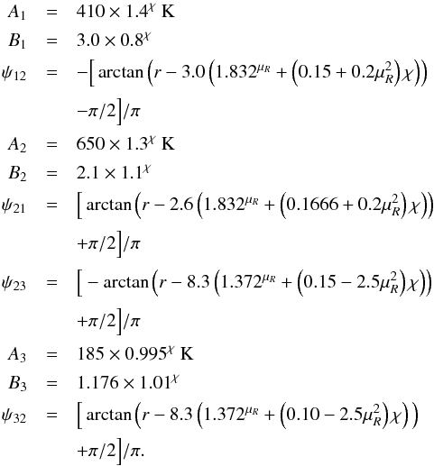 (A.7)The next regime spans the interval 8.75 × 10⁻⁹ M⊙/ yr <Ṁ ≤ 1.75 × 10⁻⁸ M⊙/yr and marks the regime where T undergoes a large change in the inner parts of the disc, because viscous heating is replaced by stellar heating as the dominant heat source. Here, Ṁref = 1.75 × 10⁻⁸ M⊙/yr (which changes μR), which results in some reduction factors R that need to be taken into account:
 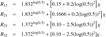 (A.8)The fit then reads as
 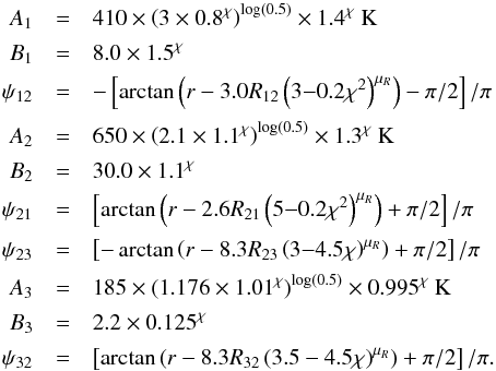 (A.9)For even lower Ṁ values, the disc is dominated by stellar heating. We therefore have to introduce another regime that is Ṁ ≤ 8.75 × 10⁻⁹ M⊙/yr. The reduction factors are now
 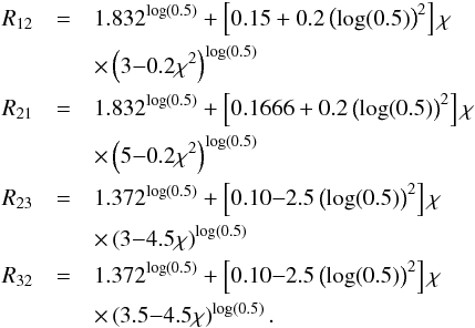 (A.10)Here Ṁref = 8.75 × 10⁻⁹ M⊙/yr and the fit reads as
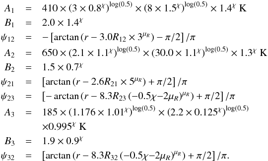 (A.11)For accretion rates of 1 × 10⁻¹⁰ M⊙/ yr <Ṁ< 1 × 10⁻⁸ M⊙/yr, photo evaporation of the disc can be dominant and clear the disc on a very short time scale (Alexander et al. 2014). This implies that going to accretion rates of Ṁ< 1 × 10⁻⁹ M⊙/yr might not be relevant for the evolution of the disc. Therefore we recommend not using these fits for Ṁ< 1 × 10⁻⁹ M⊙/yr because the disc will be photo-evaporated away in a very short time for these parameters.
In Fig. 5 the mid-plane temperature (top), H/r (middle), and the surface density (bottom) of our simulations and the fits from Eqs. (A.6) to (A.11) with Z = 0.005 are displayed (shown in black lines). The general quantities of the discs are captured well by the provided fits. In Fig. 6 the Δ parameter (Eq. (6)) of the simulations with Z = 0.005 and the one derived from the fit is displayed. The general trend towards a decreasing Δ in the inner parts of the disc with decreasing Ṁ is reproduced well. The pressure in the disc is calculated through its proportionality with the disc’s density ![]() (A.12)where cV is the specific heat at constant volume. In hydrostatic equilibrium the density is calculated through
(A.12)where cV is the specific heat at constant volume. In hydrostatic equilibrium the density is calculated through ![]() . The fit in Δ seems to be a bit off for Ṁ< 4.375 × 10⁻⁹ M⊙/yr. The reason for that lies in the different quantities that are needed to compute Δ. Small errors in independent variables (e.g. T, ΣG) translate into larger errors in the final quantity (here Δ).
. The fit in Δ seems to be a bit off for Ṁ< 4.375 × 10⁻⁹ M⊙/yr. The reason for that lies in the different quantities that are needed to compute Δ. Small errors in independent variables (e.g. T, ΣG) translate into larger errors in the final quantity (here Δ).
In Fig. 7 the torque maps for the discs with Ṁ = 7 × 10⁻⁸ M⊙/yr (top) and Ṁ = 8.75 × 10⁻⁹ M⊙/yr (bottom) with Z = 0.005 are displayed. The white lines indicate the zero-torque lines resulting from the fitted disc structures presented by the black lines in Fig. 5. The overall agreement in the torque acting on the planet from the fit compared to the simulation is quite good, but there seem to be some variations on the “edges” of the region of outward migration. This is caused by the fit having small deviations from the simulations for all quantities of the disc. But in the migration formula of Paardekooper et al. (2011), all these quantities and their gradients play a role. This is especially important for the torque saturation at higher planetary masses. However, the general trend, especially for low mass planets, is captured well.
Appendix A.2: High metallicity discs
In this section fits for discs with high metallicity (Z ≥ 0.005) are presented. The fits follow the basic principles as for the low metallicity discs, but the parameters for A, B, and ψ differ, because the dependence on Z and therefore on χ changes. The first regime of Ṁ for Ṁ> 3.5 × 10⁻⁸ M⊙/yr is represented by the following fit (where r is in units of AU) 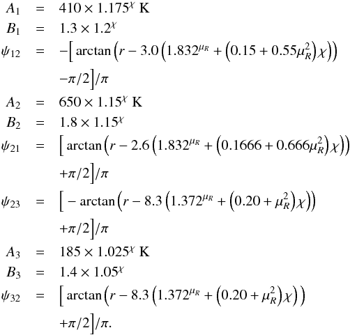 (A.13)The next regime spans the interval 1.75 × 10⁻⁸ M⊙/ yr <Ṁ ≤ 3.5 × 10⁻⁸ M⊙/yr and Ṁref = 3.5 × 10⁻⁸ M⊙/yr and the fit reads as
 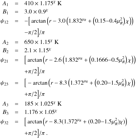 (A.14)The next regime spans the interval 8.75 × 10⁻⁹ M⊙/ yr <Ṁ ≤ 1.75 × 10⁻⁸ M⊙/yr and marks the regime where T undergoes a large change in the inner parts of the disc, because viscous heating is replaced by stellar heating as dominant heat source. Here, Ṁref = 1.75 × 10⁻⁸ M⊙/yr (which changes μR), which results in some reduction factors R that need to be taken into account:
 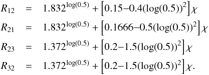 (A.15)The fit then reads
|
Fig. A.2
H/r for discs with various Ṁ and metallicity. The metallicity is 0.1% in the top panel, 1.0% in the second from top panel, 2.0% in the third from top panel, and 3.0% in the bottom panel. An increasing metallicity reduces the cooling rate of the disc, making the disc hotter, and therefore increases H/r. The black lines in the plots indicate the fit presented in Appendix A. |
|
| Open with DEXTER | |
as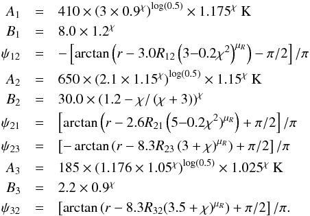 (A.16)For even lower Ṁ values, the disc is dominated by stellar heating. We therefore have to introduce another regime that is Ṁ ≤ 8.75 × 10⁻⁹ M⊙/yr. The reduction factors are now
 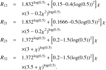 (A.17)Here Ṁref = 8.75 × 10⁻⁹ M⊙/yr and the fit reads as
 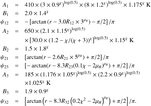 (A.18)The black lines in Fig. 8 represent the fits obtained with the formulas of Eqs. (A.13) to (A.18) for discs with different Z. In Figs. A.2 and A.3, the surface density and H/r of the same discs and the corresponding fits are displayed.
|
Fig. A.3
Surface density ΣG for discs with various Ṁ and metallicity. The metallicity is 0.1% in the top panel, 1.0% in the second from top panel, 2.0% in the third from top panel, and 3.0% in the bottom panel. An increasing metallicity reduces the cooling rate of the disc, making the disc hotter, increasing the viscosity, and therefore decreasing ΣG compared to discs with lower metallicity. The black lines in the plots indicate the fits presented in Appendix A. |
|
| Open with DEXTER | |
|
Fig. A.4
Mid-plane temperature (top), H/r (middle), and surface density ΣG (bottom) for discs at different time evolutions. The values for T, H/r, and ΣG have been calculated from Eqs. (A.6) to (A.11) with a metallicity of 0.5%. As time evolves, the surface density reduces and with it the inner region that is dominated by viscous heating, so that the disc is dominated by stellar irradiation at the late stages of the evolution, after a few Myr. In this late stage, the aspect ratio is nearly constant in the inner parts of the disc and T and ΣG follow simple power laws. |
|
| Open with DEXTER | |
Appendix A.3: Time evolution of the disc
To link these fits with time evolution, we relate back to Eq. (4), which links time with a corresponding Ṁ value. For each Ṁ value, we can calculate the disc structure through Eqs. (A.6) to (A.11) for discs with Z ≤ 0.005 and through Eqs. (A.13) to (A.18) for discs with Z> 0.5. We can therefore calculate what the disc structure looks like at different times. This is presented in Fig. A.4, where temperature (top), H/r (middle), and surface density (bottom) of discs with Z = 0.005 and different ages are displayed.
The age of the disc, tdisc = 0 is not defined in Eq. (4). Here we take the age tdisc = 0 to be 100 kyr after the formation of the disc, because during the first stages, the disc is still undergoing massive changes in its structure (Williams & Cieza 2011). We therefore recommend using this definition of tdisc = 0 age because it avoids discontinuities in the disc evolution. The age of the star, presented in Table 1, follows a different time scale, meaning age tdisc = 0 for the disc corresponds to a stellar age of t⋆ = 100 kyr. This means we add 100 kyr in Eq. (4) to define the new tdisc = 0 age for the disc in the time of the star. Equation (4) then looks (without the measurement errors): 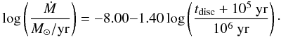 (A.19)This equation describes the age of the disc tdisc in our set-up (indicated in Fig. A.4), while Eq. (4) describes the age of the star t⋆ as stated in Table 1.
© ESO, 2015
Current usage metrics show cumulative count of Article Views (full-text article views including HTML views, PDF and ePub downloads, according to the available data) and Abstracts Views on Vision4Press platform.
Data correspond to usage on the plateform after 2015. The current usage metrics is available 48-96 hours after online publication and is updated daily on week days.
Initial download of the metrics may take a while.