| Issue |
A&A
Volume 574, February 2015
|
|
|---|---|---|
| Article Number | A110 | |
| Number of page(s) | 10 | |
| Section | Extragalactic astronomy | |
| DOI | https://doi.org/10.1051/0004-6361/201424729 | |
| Published online | 03 February 2015 | |
Online material
Appendix A
We derived four independent methods of estimating the relation between magnetic field (B) and particle density (K) for the simple SSC model used in this work. In addition we provide a simple method of constraining the magnetic field value.
Appendix A.1: Synchrotron peak
According to our assumption, the particle energy distribution is described by a power-law function ![]() (A.1)For such a simple distribution, the synchrotron emissivity in the source’s comoving frame can also be approximated by a power-law relation
(A.1)For such a simple distribution, the synchrotron emissivity in the source’s comoving frame can also be approximated by a power-law relation 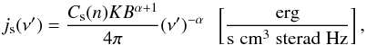 (A.2)where α = (n − 1)/2 and the coefficient
 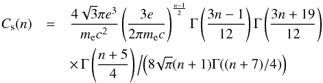 (A.3)(e.g. Ginzburg & Syrovatskii 1965). The coefficient above is quite complex. However, it can be approximated very well by a simple polynomial formula
 ![]() (A.4)that is precise enough (ΔCs< 2% for 1.5 ≤ n ≤ 4) for our estimations. All the formulas we present in this appendix are universal, applicable for any synchrotron and/or SSC source. Therefore, our goal was to provide as simple equations as possible. In all the cases we provide a simple polynomial approximation of more complex coefficients.
(A.4)that is precise enough (ΔCs< 2% for 1.5 ≤ n ≤ 4) for our estimations. All the formulas we present in this appendix are universal, applicable for any synchrotron and/or SSC source. Therefore, our goal was to provide as simple equations as possible. In all the cases we provide a simple polynomial approximation of more complex coefficients.
The intensity of the surface emission of spherical, optically thin source is given by ![]() (A.5)and the flux is defined by
(A.5)and the flux is defined by 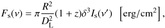 (A.6)where: δ is the Doppler factor, z the redshift, DL the luminosity distance. The frequency transformation is given by ν = ν′δ/ (1 + z). Using these formulae we may write our first B → K relation
 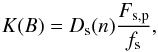 (A.7)where
  (A.8)and
 ![]() (A.9)is the correction coefficient. We use a simple power-law approximation of the synchrotron spectrum that differs from precisely calculated spectrum, especially at the νFs(ν) peak, where the precise spectrum has a curved shape. Therefore, it is necessary to introduce an adequate correction. We have calculated the difference between the precise and the approximated spectrum for different values of n (1.5 ≤ n< 3) and expressed this difference by the polynomial presented above. We note that Fs,p and νs,p are observable quantities, the Doppler factor in all our estimations is assumed to be δ = 1, and the radius is constrained from the radio maps.
(A.9)is the correction coefficient. We use a simple power-law approximation of the synchrotron spectrum that differs from precisely calculated spectrum, especially at the νFs(ν) peak, where the precise spectrum has a curved shape. Therefore, it is necessary to introduce an adequate correction. We have calculated the difference between the precise and the approximated spectrum for different values of n (1.5 ≤ n< 3) and expressed this difference by the polynomial presented above. We note that Fs,p and νs,p are observable quantities, the Doppler factor in all our estimations is assumed to be δ = 1, and the radius is constrained from the radio maps.
Appendix A.2: Inverse-Compton peak
The inverse-Compton emissivity in our simple SSC scenario can also be approximated by a power-law function ![]() (A.10)where log 10(Cc) = 6.58 × 10⁻⁴α − 46.2. This approximation is valid only in the Thompson regime of the scattering. The intensity, flux, and frequency transformations are identical as in the case of the synchrotron emission. Thus, second B → K relation is
(A.10)where log 10(Cc) = 6.58 × 10⁻⁴α − 46.2. This approximation is valid only in the Thompson regime of the scattering. The intensity, flux, and frequency transformations are identical as in the case of the synchrotron emission. Thus, second B → K relation is  (A.11)where by analogy
 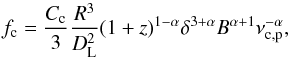 (A.12)and the correction coefficient is given by
 ![]() (A.13)The other assumptions for this estimation are identical, as in the case of the synchrotron emission.
(A.13)The other assumptions for this estimation are identical, as in the case of the synchrotron emission.
Appendix A.3: Equipartition
The other relation was derived from the assumption about the equipartition (UB = Ue) between the magnetic field energy density  (A.14)and the particle energy density
 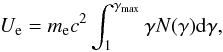 (A.15)which gives
 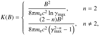 (A.16)where the Lorentz factor that characterize the maximal energy of the particles was obtained from the synchrotron peak frequency
  (A.17)where Ps(n) = −1.9 × 10⁵n3 + 8.4 × 10⁵n2 − 1.9 × 10⁶n + 3.5 × 10⁶ was obtained for the specific case of the synchrotron peak created by an abrupt cutoff in the particle energy distribution (Eq. (A.1)).
Appendix A.4: Self-absorption frequency
We assumed that the source is optically thin (Eq. (A.5)) at the frequencies (IR to X-ray) where the peaks are observed. This is very reasonable assumption that simplifies the calculations. However, at radio frequencies, the synchrotron self-absorption process may drastically change the slope of the spectrum. The low-frequency, self-absorbed emission will have a constant slope α = 5/2, whereas the spectral index of the optically thin part will depend on the particle energy slope (α = (n − 1)/2). This gives a characteristic break in the spectrum at the frequency that depends on B,K,R. The coefficient that describes the absorption for the source with a power-law particle energy distribution can also be approximated by a power law formula ![]() (A.18)where log 10(Bs) = 0.14n2 + 2.43n + 6 for 1.5 ≤ n ≤ 4. Assuming that at the break frequency (νs,b) the optical depth (τ = Rks) is equal unity, we may obtain another relation between B and K
(A.18)where log 10(Bs) = 0.14n2 + 2.43n + 6 for 1.5 ≤ n ≤ 4. Assuming that at the break frequency (νs,b) the optical depth (τ = Rks) is equal unity, we may obtain another relation between B and K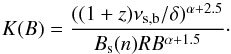 (A.19)
Appendix A.5: Relative peak positions
Finally, a simple constraint for only the magnetic field can be obtained from the formula (A.17)  (A.20)where this time
 ![]() and Pc(n) = −0.48n + 1.3. The maximum energy (γmax) was derived from relative position of the peaks. According to the basic theory of the IC scattering, on average
and Pc(n) = −0.48n + 1.3. The maximum energy (γmax) was derived from relative position of the peaks. According to the basic theory of the IC scattering, on average ![]() . However, our simulations show that in the case of simple power-law particle energy distribution with a sharp cut-of, f it is more precise to use the coefficient Pc that depends on the slope instead of the factor 4/3, in the above formulae.
. However, our simulations show that in the case of simple power-law particle energy distribution with a sharp cut-of, f it is more precise to use the coefficient Pc that depends on the slope instead of the factor 4/3, in the above formulae.
© ESO, 2015
Current usage metrics show cumulative count of Article Views (full-text article views including HTML views, PDF and ePub downloads, according to the available data) and Abstracts Views on Vision4Press platform.
Data correspond to usage on the plateform after 2015. The current usage metrics is available 48-96 hours after online publication and is updated daily on week days.
Initial download of the metrics may take a while.