| Issue |
A&A
Volume 574, February 2015
|
|
|---|---|---|
| Article Number | L4 | |
| Number of page(s) | 6 | |
| Section | Letters | |
| DOI | https://doi.org/10.1051/0004-6361/201424718 | |
| Published online | 22 January 2015 | |
Online material
Appendix A: CASSIS LTE modeling
CASSIS provides a Jython script which minimizes the χ2 to find the best parameters to adjust the observations. With a spectrum i of N points, the χ2 is derived as 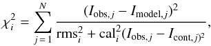 where Iobs and Imodel are respectively the observed and the modeled intensities, Icont is the continuum intensity, cali the calibration uncertainty for the spectrum i and N is the total number of points of the spectrum. The reduced χ2 is the calculated as
 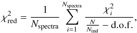 with Nspectra the number of spectra, Nind the number of independent points, and dof the degree of freedom.
The adjustable parameters are the column density, temperature, FWHM, size of the source, and vLSR. In the case of CF+, the column density varies between 1010 and 1014 cm-2 with 500 steps; the other parameters were fixed. The temperature was set to 10 K, as in Neufeld et al. (2006) and Guzmán et al. (2012). The FWHM was measured on the spectrum as 1.6 km s-1. No source size was assumed, so we kept the 30 m beam size of 25′′. The velocity of the source is around − 4 km s-1. CASSIS also takes into account the beam size variation as a function of the frequency. The obtained ![]() is 3.22 and the column density is (4 ± 1) × 1011 cm-2.
is 3.22 and the column density is (4 ± 1) × 1011 cm-2.
The VLSR and FWHM derived for the J = 1−0 line are then used to predict the intensity of the J = 2−1 line. We detected 202 CH3CHO lines in the whole coverage and used a population diagram to derive a mean excitation temperature of 40 K and a column density of 3 × 1013 cm-2. These values were used to model the CH3CHO lines as shown in the bottom panel of Fig. 1.
Appendix B: VLA observations
CygX-N63 was observed on 27 April 2003 with the 27 antennas of the VLA in D configuration at 8.4 GHz (band X) (project AB1073). The image shown in Fig. B.1 corresponds to a total integration time of 25 mins spread over 4.5 h (track sharing technique to improve UV coverage). It has been cleaned with the clean algorithm of AIPS. The resulting rms is equal to 60.2 μJy/beam.
In the direction of CygX-N63, a weak peak of 0.14mJy, i.e. at a level of 2.3σ, is found. Below 3σ it cannot be considered as a possible detection, especially because the side lobes (large stripes in the image of Fig. B.1) are roughly of the same intensity.
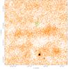 |
Fig. B.1
VLA image at 8.4 GHz of the same region than in Fig. 2 with color scale from − 0.1 to 0.7 mJy/beam. The dashed ellipse indicates the VLA primary beam and the green circle shows the IRAM 30 m beam at 102 GHz. The rms in this image stays large, of the order of 0.06 mJy/beam, due to strong sidelobes originating from to DR22, a strong radio source (a compact HII region) outside the imaged field (~5 arcmin south). |
| Open with DEXTER | |
Appendix C: Carbon ionization equilibrium
At equilibrium in spherical geometry from an initial radius ri to the radius of the CII region (where mostly all carbons are ionized) rCII the equilibrium of carbon ionization can be expressed as 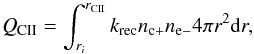 where QCII is the total rate of ionizing photons (in s-1), krec is the carbon recombination rate that we take as equal to 2.36 × 10⁻¹²(T/ 300)-0.29 exp(− 17.7 /T) cm3s-1 (UMIST 2012 database McElroy et al. 2013), and nc + and ne − are the densities of C+ and of electrons. For a large range of gas temperature (10 to 4000 K), krec stays within a factor of less than 2 around the adopted value of 1.74 × 10⁻¹²s-1 (ranging from 1.08 to 2.80 × 10⁻¹²s-1 with the maximum obtained at ~60 K).
If carbon ionization dominates and assuming C+/H equal to the standard C/H ratio of 1.6 × 10⁻⁴ (if most of the carbon is in atomic form), we have ne − = nC + = 1.6 × 10⁻⁴ × nH. Assuming a r-2 density law and having 44.3 M⊙ inside a FWHM of 2500 AU (Duarte-Cabral et al. 2013), we here get an H2 density of 1.95 × 10¹⁰ × (r/ 100 AU)-2cm-3. For this simple model, we get the following expression of the extent of the ionized region in the inner envelope, 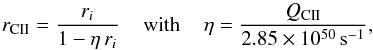 and the radii expressed in AU. For the case of Sect. 4.3 (QCII = 2.63 × 1045s-1), one gets a very small value of 9.4 × 10⁻⁶ for η. For ri = 100 AU, rCII is then equal to 100.1 AU. Only the very first layers are ionized for values of QCII significantly lower than ~1050s-1.
The ionization equilibrium can also be expressed as 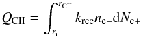 with Nc + being the number of ionized carbons. It shows that krecne − is the fraction of ionized carbons that recombines per second. For ne − = 1.6 × 10⁻⁴ × nH, we can then derive the typical density (assuming constant density) required to keep an amount of ionized carbon Nc + ionized under an ionizing rate QCII. Here is the expression of this density nHCII for our adopted numerical values:
 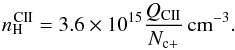 For the case of Sect. 4.3 with QCII = 2.63 × 1045s-1 and Nc + = 1.2 × 1053, one gets nHCII = 7.9 × 107cm-3.
Appendix D: Centimetric free-free emission
As discussed in Sect. 4.6, any ionized gas is expected to emit free-free emission.
The centimetric flux of free-free emission in the optically thin case can be expressed as a function of EMV, the emission measure (see André 1987; Curiel et al. 1987), 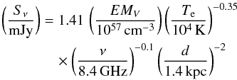 with
with  The optical depth is expressed as a function of the linear emission measure EML (
![]() ),
),
 which is equal to ~8.8 × 10⁶ for ne − = nH = 2.2 × 109cm-3, l = 100 AU (see Sect. 4.4), 104K (the opacity is even larger for lower temperatures) and at 8.4 GHz (frequency of the VLA observation from Appendix B).
In the optically thick case the emission depends on the area of emission expressed in physical surface Aem if distance scaling is included,  which is equal to 0.3 mJy for Aem = πRem2 with Rem = 19.2 AU (Sect. 4.4).
Curiel et al. (1987, 1989) also expressed the expected flux and optical depth in the case of a dissociative shock as a function of pre-shock density n0 and shock velocity Vs (for Vs ≳ 60 km s-1),  which is found equal to 5 × 10⁻⁴ for n0 = 3 × 10⁻³cm-3, Vs = 200 km s-1 (see Sect. 4.5), 104K and at 8.4 GHz.
© ESO, 2015
Current usage metrics show cumulative count of Article Views (full-text article views including HTML views, PDF and ePub downloads, according to the available data) and Abstracts Views on Vision4Press platform.
Data correspond to usage on the plateform after 2015. The current usage metrics is available 48-96 hours after online publication and is updated daily on week days.
Initial download of the metrics may take a while.