| Issue |
A&A
Volume 567, July 2014
|
|
|---|---|---|
| Article Number | A50 | |
| Number of page(s) | 18 | |
| Section | Interstellar and circumstellar matter | |
| DOI | https://doi.org/10.1051/0004-6361/201423614 | |
| Published online | 09 July 2014 | |
Online material
Appendix A: General solution of the transport equation
In order to find a general solution of the transport Eq. (1) using Green’s method, first the fundamental solution
G(r,p,t |
r0,p0,t0),
that is, the solution for the Dirac source distribution
 is
determined.The fundamental transport equation is then given by
is
determined.The fundamental transport equation is then given by 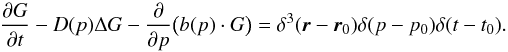 (28)In terms of the
function R(r,p,t) =
b(p)·G(r,p,t),
Eq. (28) becomes
(28)In terms of the
function R(r,p,t) =
b(p)·G(r,p,t),
Eq. (28) becomes 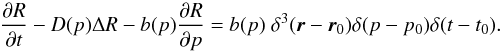 (29)With the new
coordinate
(29)With the new
coordinate 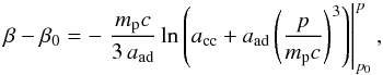 (30)induced by
∂β = −
b(p)∂p,
and δ(β −
β0) =
b(p0)·δ(p
− p0), Eq. (29) yields
(30)induced by
∂β = −
b(p)∂p,
and δ(β −
β0) =
b(p0)·δ(p
− p0), Eq. (29) yields 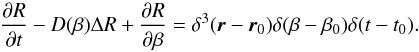 (31)This partial
differential equation can be solved by first applying a Laplace transformation
L[·] with respect to the
time variable t
(31)This partial
differential equation can be solved by first applying a Laplace transformation
L[·] with respect to the
time variable t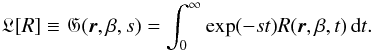 (32)Note that the lower
integration limit in the definition of the Laplace transformation (32) fixes t0 = 0 without
loss of generality. The Laplace transform of Eq. (31) reads
(32)Note that the lower
integration limit in the definition of the Laplace transformation (32) fixes t0 = 0 without
loss of generality. The Laplace transform of Eq. (31) reads  (33)Since
R is
related linearly to the differential CR proton number density, R ∝ dN/
dV, where N is the (finite) number
of protons, and V is the volume within which the protons are
distributed, this function vanishes at t = 0, because the distribution of CR protons at
this time is restricted to the boundary r =
r0 of the MC. Then, Eq.
(33) reduces to the inhomogeneous,
linear partial differential equation of first order in β and second order in
r,
(33)Since
R is
related linearly to the differential CR proton number density, R ∝ dN/
dV, where N is the (finite) number
of protons, and V is the volume within which the protons are
distributed, this function vanishes at t = 0, because the distribution of CR protons at
this time is restricted to the boundary r =
r0 of the MC. Then, Eq.
(33) reduces to the inhomogeneous,
linear partial differential equation of first order in β and second order in
r, 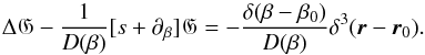 (34)This equation can be
solved explicitly by using Duhamel’s principle (Duhamel
1838; Courant & Hilbert 2008),
which is a general method to find solutions of inhomogeneous, linear partial
differential equations in terms of the solutions of the Cauchy problems for the
corresponding homogeneous partial differential equations, that is, by interpreting the
inhomogeneity as a boundary value condition in a higher-dimensional space labeled with
an additional auxiliary variable. This principle is applied here on a linear partial
differential equation with a product-separable inhomogeneity of single-variable factors
with respect to the variables r and β,
(34)This equation can be
solved explicitly by using Duhamel’s principle (Duhamel
1838; Courant & Hilbert 2008),
which is a general method to find solutions of inhomogeneous, linear partial
differential equations in terms of the solutions of the Cauchy problems for the
corresponding homogeneous partial differential equations, that is, by interpreting the
inhomogeneity as a boundary value condition in a higher-dimensional space labeled with
an additional auxiliary variable. This principle is applied here on a linear partial
differential equation with a product-separable inhomogeneity of single-variable factors
with respect to the variables r and β,  (35)where
 (36)From the structure of
the left-hand side of Eq. (35), it
directly follows that the solution of the corresponding homogeneous equation is
product-separable Ghom =
S(r)P(β,s).
An embedding of the original (r,β,s)-space
into the extended, higher-dimensional (r,β,s,u)-space,
where
(36)From the structure of
the left-hand side of Eq. (35), it
directly follows that the solution of the corresponding homogeneous equation is
product-separable Ghom =
S(r)P(β,s).
An embedding of the original (r,β,s)-space
into the extended, higher-dimensional (r,β,s,u)-space,
where  , implies
that there is a family of functions Su(r): =
S(r,u)
and Pu(β,s): =
P(β,s,u), fulfilling the
relations ÔrS(r,u)
=
∂uS(r,u)
and Ôβ,sP(β,s,u)
=
∂uP(β,s,u)
with the boundary conditions
, implies
that there is a family of functions Su(r): =
S(r,u)
and Pu(β,s): =
P(β,s,u), fulfilling the
relations ÔrS(r,u)
=
∂uS(r,u)
and Ôβ,sP(β,s,u)
=
∂uP(β,s,u)
with the boundary conditions  (37)such that the full,
non-trivial solution of Eq. (35) is
given by the integral
(37)such that the full,
non-trivial solution of Eq. (35) is
given by the integral 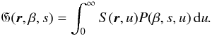 (38)Technically, this
integral represents the “summation” over the entire family of homogeneous solutions in
the extended coordinate space with boundary conditions compatible with the
inhomogeneity. Within this setting, Eq. (34) decouples into the simpler set of partial differential equations
(38)Technically, this
integral represents the “summation” over the entire family of homogeneous solutions in
the extended coordinate space with boundary conditions compatible with the
inhomogeneity. Within this setting, Eq. (34) decouples into the simpler set of partial differential equations
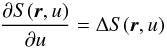 (39)and
 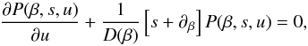 (40)which has to be solved
in order to determine the fundamental solution G via the integral in Eq. (38). The solution of Eq. (39) is the well-known heat kernel of
three-dimensional Euclidean space
(40)which has to be solved
in order to determine the fundamental solution G via the integral in Eq. (38). The solution of Eq. (39) is the well-known heat kernel of
three-dimensional Euclidean space 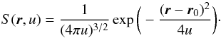 (41)A solution of Eq.
(40) can directly be found after
performing a Laplace transformation with respect to the variable u
(41)A solution of Eq.
(40) can directly be found after
performing a Laplace transformation with respect to the variable u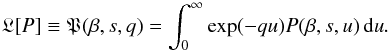 (42)Then, Eq. (40) becomes
 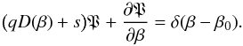 (43)Note that the
boundary condition P(β,s,u = 0) =
δ(β − β0)
/D(β) was
already fixed in (37). Using an
integrating factor of the form
(43)Note that the
boundary condition P(β,s,u = 0) =
δ(β − β0)
/D(β) was
already fixed in (37). Using an
integrating factor of the form 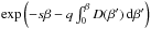 ,
Eq. (43) can be rewritten as
,
Eq. (43) can be rewritten as
 (44)and
solved by simple integration, leading to
(44)and
solved by simple integration, leading to
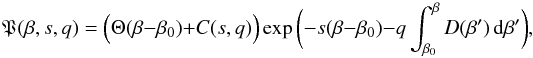 (45)where Θ(·) is the Heaviside step function and
C(s,q) is an integration constant
with respect to β. Since only momentum-loss processes are
considered, there are no particles with momenta larger than their initial momentum
p>p0,
corresponding to β<β0,
at any time. Therefore, because the function S(r,u)
is independent of β, P(β,s,q) must vanish for β<β0
implying C(s,q) = 0. Then, the solution
of Eq. (43) reads
(45)where Θ(·) is the Heaviside step function and
C(s,q) is an integration constant
with respect to β. Since only momentum-loss processes are
considered, there are no particles with momenta larger than their initial momentum
p>p0,
corresponding to β<β0,
at any time. Therefore, because the function S(r,u)
is independent of β, P(β,s,q) must vanish for β<β0
implying C(s,q) = 0. Then, the solution
of Eq. (43) reads 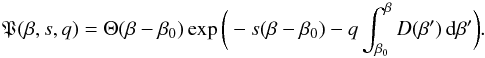 (46)Via an inverse
Laplace transformation with respect to the variable q, one can recover the
function P(β,s,u)
(46)Via an inverse
Laplace transformation with respect to the variable q, one can recover the
function P(β,s,u)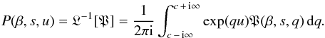 (47)Since
P is well-defined and
finite everywhere, one is free to choose the real-valued constant c = 0. Therefore, from
using the relation
(47)Since
P is well-defined and
finite everywhere, one is free to choose the real-valued constant c = 0. Therefore, from
using the relation 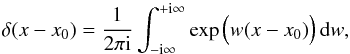 (48)it directly follows
that
(48)it directly follows
that 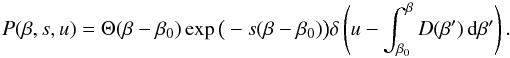 (49)Substituting the
functions (41) and (49) into the integral in Eq. (38) leads to
(49)Substituting the
functions (41) and (49) into the integral in Eq. (38) leads to
 (50)Because
 , integration with respect
to the variable u yields
, integration with respect
to the variable u yields 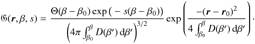 (51)In order to obtain
R(r,β,t)
from G(r,β,s), another
inverse Laplace transformation, now with respect to the variable s, is
performed,
(51)In order to obtain
R(r,β,t)
from G(r,β,s), another
inverse Laplace transformation, now with respect to the variable s, is
performed,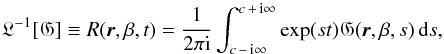 (52)where again
c = 0 is
chosen, resulting in
(52)where again
c = 0 is
chosen, resulting in 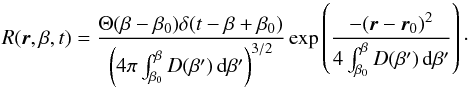 (53)The Green’s function
becomes
(53)The Green’s function
becomes 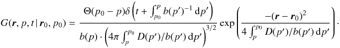 (54)The general solution
np(r,p,t)
of the transport Eq. (1), with a
momentum-loss rate given by Eq. (12) and
for an arbitrary source function Q, can be obtained by convolving the fundamental
solution G(r,p,t |
r0,p0)
with a source term Q(r0,p0,t0),
(54)The general solution
np(r,p,t)
of the transport Eq. (1), with a
momentum-loss rate given by Eq. (12) and
for an arbitrary source function Q, can be obtained by convolving the fundamental
solution G(r,p,t |
r0,p0)
with a source term Q(r0,p0,t0),
 (55)This differential CR
proton number density can also be applied to many other astrophysical situations with
scalar, momentum-dependent diffusion and any type of momentum losses, such as stellar
winds, CR diffusion in the interstellar medium, or gamma-ray bursts.
(55)This differential CR
proton number density can also be applied to many other astrophysical situations with
scalar, momentum-dependent diffusion and any type of momentum losses, such as stellar
winds, CR diffusion in the interstellar medium, or gamma-ray bursts.
Appendix B: Specific source function for SNR-MC systems
The source function Q(r0,p0,t0)
is modeled for four specific SNRs associated with MCs showing gamma-ray emission for
which data samples from spectral measurements in the X-ray energy range exist. Here, the
source spectrum is assumed to be of the specific form  (56)where
Qnorm denotes a normalization constant,
Qp(p0)
is the spectral shape of the low-energy CR protons in terms of the particle momentum
p0, and lc
characterizes the extent of the emission region. A source function of this type
describes emission that is constant over a period of time (normalized to the unit time
interval of one second) from a cubic emission volume, seen by an observer located at the
center of a face of the emission volume that coincides with the cloud surface, with a
coordinate system such that the positive Cartesian z-axis is normal to this
face and points into the cloud. The cubic geometry is chosen over the more physical,
spherical geometry for numerical feasibility. The volume of the cube-shaped emission
region,
(56)where
Qnorm denotes a normalization constant,
Qp(p0)
is the spectral shape of the low-energy CR protons in terms of the particle momentum
p0, and lc
characterizes the extent of the emission region. A source function of this type
describes emission that is constant over a period of time (normalized to the unit time
interval of one second) from a cubic emission volume, seen by an observer located at the
center of a face of the emission volume that coincides with the cloud surface, with a
coordinate system such that the positive Cartesian z-axis is normal to this
face and points into the cloud. The cubic geometry is chosen over the more physical,
spherical geometry for numerical feasibility. The volume of the cube-shaped emission
region,  , is
adapted to the spherical emission volume used in the modeling process of the gamma rays
in Sect. 4. For the specific source function (56), the integrations with respect to
r0, p0, and
t0, that have to be performed in order
to determine the differential CR proton number density (55),
, is
adapted to the spherical emission volume used in the modeling process of the gamma rays
in Sect. 4. For the specific source function (56), the integrations with respect to
r0, p0, and
t0, that have to be performed in order
to determine the differential CR proton number density (55), 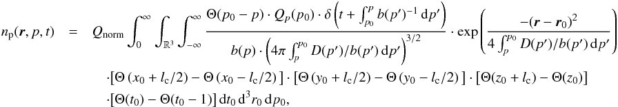 (57)can
be done separately. The specific expressions for the actual spectral shapes
Qp(p0)
and the normalization constants Qnorm used for the astrophysical
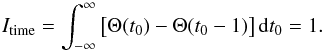
objects of interest are of no relevance for these integrations. Since the Green’s
function G(r,p,t |
r0,p0)
is independent of t0, only the time-dependent factor of
the source function, Qtime(t0) =
Θ(t0) − Θ(t0 −
1) has to be integrated with respect to t0, yielding
(57)can
be done separately. The specific expressions for the actual spectral shapes
Qp(p0)
and the normalization constants Qnorm used for the astrophysical
objects of interest are of no relevance for these integrations. Since the Green’s
function G(r,p,t |
r0,p0)
is independent of t0, only the time-dependent factor of
the source function, Qtime(t0) =
Θ(t0) − Θ(t0 −
1) has to be integrated with respect to t0, yielding
 (58)The spatial
integration
(58)The spatial
integration 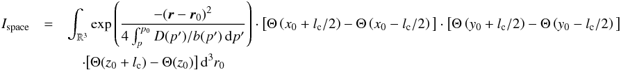 (59)results
in a product of error functions
(59)results
in a product of error functions 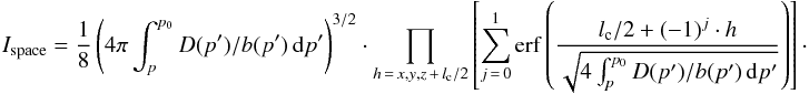 (60)Then,
one finds the following momentum integral
(60)Then,
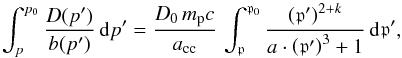
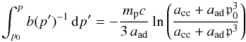
one finds the following momentum integral  (61)In
order to solve this integral, first, one has to explicitly evaluate the integrals in the
arguments of the Dirac distribution and the error functions, respectively. Starting with
the integral
(61)In
order to solve this integral, first, one has to explicitly evaluate the integrals in the
arguments of the Dirac distribution and the error functions, respectively. Starting with
the integral 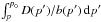 ,
keeping the solution as general as possible, the momentum dependence of the diffusion
coefficient is assumed to be
,
keeping the solution as general as possible, the momentum dependence of the diffusion
coefficient is assumed to be 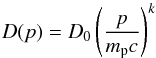 (62)with
D0 =
const. and values 1/3 ≤ k ≤ 4
/3. Using Eq. (12) and the dimensionless quantity p≡ p/
(mpc), one obtains
(62)with
D0 =
const. and values 1/3 ≤ k ≤ 4
/3. Using Eq. (12) and the dimensionless quantity p≡ p/
(mpc), one obtains
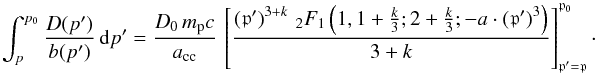
 (63)where a =
aad/acc.
An analytic solution of this integral can be found in Gradshteyn & Ryzhik (1965,
formula 3.914 number 5), yielding
(63)where a =
aad/acc.
An analytic solution of this integral can be found in Gradshteyn & Ryzhik (1965,
formula 3.914 number 5), yielding
 (64)Here,
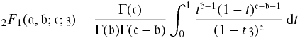 denotes
the hypergeometric function and
denotes
the hypergeometric function and 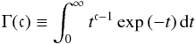 the
complete Gamma function. Substituting this and
the
complete Gamma function. Substituting this and
 (65)into
Eq. (61), one finds
(65)into
Eq. (61), one finds 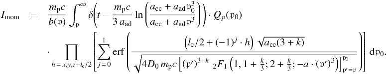 (66)The
zeros of the argument of the Dirac distribution, as a function of the momentum
p0, are given
by
(66)The
zeros of the argument of the Dirac distribution, as a function of the momentum
p0, are given
by 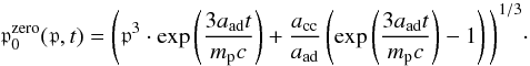 (67)Hence, the Dirac
distribution can be written as
(67)Hence, the Dirac
distribution can be written as 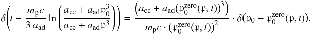 (68)Subsequently,
the momentum integral becomes
(68)Subsequently,
the momentum integral becomes  (69)Note
that
(69)Note
that  for all values of
 and
p. Then, combining of
(58), (60) and (69) leads
to the differential CR proton number density of a cubic emission source region with edge
length lc for all positions r inside the
MC, with z ≥
0, at any time t ≥ 0 and for all particle momenta
p∈ [ 0.15, 0.86 ] ≤
p0
and
p. Then, combining of
(58), (60) and (69) leads
to the differential CR proton number density of a cubic emission source region with edge
length lc for all positions r inside the
MC, with z ≥
0, at any time t ≥ 0 and for all particle momenta
p∈ [ 0.15, 0.86 ] ≤
p0 (70)
(70)
© ESO, 2014
Current usage metrics show cumulative count of Article Views (full-text article views including HTML views, PDF and ePub downloads, according to the available data) and Abstracts Views on Vision4Press platform.
Data correspond to usage on the plateform after 2015. The current usage metrics is available 48-96 hours after online publication and is updated daily on week days.
Initial download of the metrics may take a while.