| Issue |
A&A
Volume 567, July 2014
|
|
|---|---|---|
| Article Number | A85 | |
| Number of page(s) | 14 | |
| Section | The Sun | |
| DOI | https://doi.org/10.1051/0004-6361/201321973 | |
| Published online | 16 July 2014 | |
Online material
Appendix A: Electron beam instability
We initially assume a one dimensional electron beam injected at height r = 0 of the form (see
Reid et al. 2011)  (A.1)where
g0(v) ∝ v−
α and α is the spectral index
of the electron beam (in velocity space). d is the characteristic size of the electron beam
(and consequently the size of the acceleration region). At t>
0 the electron beam propagates through space (reaching distance
vt1 at time
t1), creating a bump-in-tail
distribution that causes resonant Langmuir wave growth as ∂f/∂v>
0 (Drummond & Pines
1962; Vedenov et al. 1962). The Langmuir
wave quasilinear growth rate γ(v,r) and the collisional
absorption of Langmuir waves γc are given by
(A.1)where
g0(v) ∝ v−
α and α is the spectral index
of the electron beam (in velocity space). d is the characteristic size of the electron beam
(and consequently the size of the acceleration region). At t>
0 the electron beam propagates through space (reaching distance
vt1 at time
t1), creating a bump-in-tail
distribution that causes resonant Langmuir wave growth as ∂f/∂v>
0 (Drummond & Pines
1962; Vedenov et al. 1962). The Langmuir
wave quasilinear growth rate γ(v,r) and the collisional
absorption of Langmuir waves γc are given by 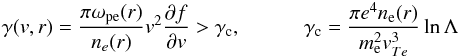 (A.2)where
lnΛ is the Coulomb
logarithm, taken as 20 for the parameters in the corona. ωpe(r), ne(r) and
vTe are the background plasma frequency,
density and thermal velocity respectively. When the growth of Langmuir waves becomes
larger than the collisional absorption of Langmuir waves from the background plasma we
can obtain Langmuir waves orders of magnitude above thermal levels. Radio waves can then
be produced through wave-wave interactions at the local plasma frequency and the
harmonics, which we observe as type III radio bursts (e.g. Kontar & Pécseli 2002; Li et
al. 2008).
(A.2)where
lnΛ is the Coulomb
logarithm, taken as 20 for the parameters in the corona. ωpe(r), ne(r) and
vTe are the background plasma frequency,
density and thermal velocity respectively. When the growth of Langmuir waves becomes
larger than the collisional absorption of Langmuir waves from the background plasma we
can obtain Langmuir waves orders of magnitude above thermal levels. Radio waves can then
be produced through wave-wave interactions at the local plasma frequency and the
harmonics, which we observe as type III radio bursts (e.g. Kontar & Pécseli 2002; Li et
al. 2008).
At time t> 0 we can describe the
distribution function assuming no energy loss using
 (A.3)and
the growth rate for Langmuir waves becomes
(A.3)and
the growth rate for Langmuir waves becomes 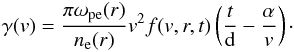 (A.4)Langmuir
waves will occur at a height htypeIII which can be found at a
distance Δr =
htypeIII −
hacc from the acceleration site at
hacc. Using the condition that Langmuir
waves will be prolific when the growth rate exceeds the collisional absorption rate we
can find the distance Δr via
(A.4)Langmuir
waves will occur at a height htypeIII which can be found at a
distance Δr =
htypeIII −
hacc from the acceleration site at
hacc. Using the condition that Langmuir
waves will be prolific when the growth rate exceeds the collisional absorption rate we
can find the distance Δr via 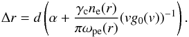 (A.5)The
second term in the brackets can be approximated using coronal parameters. We can use
vg0(v) =
nb were nb is the
electron beam density. We assume ne(r) = 109
cm-3, Te = 2 MK, nb = 104
cm and we find that this term is around 10-3 ≪ α. Thus
we find the simple relation
(A.5)The
second term in the brackets can be approximated using coronal parameters. We can use
vg0(v) =
nb were nb is the
electron beam density. We assume ne(r) = 109
cm-3, Te = 2 MK, nb = 104
cm and we find that this term is around 10-3 ≪ α. Thus
we find the simple relation 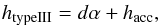 (A.6)that
equates the known quantities htypeIII and α we can deduce from
observations to the unknown quantities of d,
(A.6)that
equates the known quantities htypeIII and α we can deduce from
observations to the unknown quantities of d,
the vertical extent of the acceleration region and hacc the height of the acceleration region.
Appendix B: Isotropic electron beam instability
We now assume an initial electron beam that can vary with pitch angle such that at
t = 0 we
inject  (B.1)where
ψ(μ) is the pitch angle
distribution and
(B.1)where
ψ(μ) is the pitch angle
distribution and  . We consider an initial
isotropic distribution function where ψ(μ) = const at t = 0. Again
g0(v) ∝ v−
α and α is then spectral index
of the electron beam (in velocity space). d is the characteristic size of the electron beam
(and consequently the size of the acceleration region). The distribution function at
t>
0 becomes
. We consider an initial
isotropic distribution function where ψ(μ) = const at t = 0. Again
g0(v) ∝ v−
α and α is then spectral index
of the electron beam (in velocity space). d is the characteristic size of the electron beam
(and consequently the size of the acceleration region). The distribution function at
t>
0 becomes  (B.2)where
v is the
speed of the electrons. We can find the reduced distribution along B using
(B.2)where
v is the
speed of the electrons. We can find the reduced distribution along B using 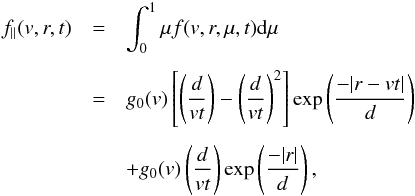 (B.3)where
we integrated for r −
vμt> 0 as we are
interested in the growing part of the electron beam where ∂f/∂v>
0. Assuming that r ≫ d and d/vt ≪
1, as predicted by Eq. (2), we can approximate Eq. (B.3) as
(B.3)where
we integrated for r −
vμt> 0 as we are
interested in the growing part of the electron beam where ∂f/∂v>
0. Assuming that r ≫ d and d/vt ≪
1, as predicted by Eq. (2), we can approximate Eq. (B.3) as 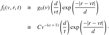 (B.4)By
finding ∂f∥/∂v
we obtain the equation for the growth rate of Langmuir waves
(B.4)By
finding ∂f∥/∂v
we obtain the equation for the growth rate of Langmuir waves
 (B.5)Using
the same analysis demonstrated between Eqs. (A.4) and (A.6) we find the
simple relation
(B.5)Using
the same analysis demonstrated between Eqs. (A.4) and (A.6) we find the
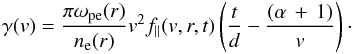
simple relation  (B.6)that
equates the known quantities htypeIII and α we can deduce from
observations to the unknown quantities of d, the vertical extent of the acceleration region
and hacc the height of the acceleration
region.
(B.6)that
equates the known quantities htypeIII and α we can deduce from
observations to the unknown quantities of d, the vertical extent of the acceleration region
and hacc the height of the acceleration
region.
© ESO, 2014
Current usage metrics show cumulative count of Article Views (full-text article views including HTML views, PDF and ePub downloads, according to the available data) and Abstracts Views on Vision4Press platform.
Data correspond to usage on the plateform after 2015. The current usage metrics is available 48-96 hours after online publication and is updated daily on week days.
Initial download of the metrics may take a while.