| Issue |
A&A
Volume 562, February 2014
|
|
|---|---|---|
| Article Number | A71 | |
| Number of page(s) | 28 | |
| Section | Galactic structure, stellar clusters and populations | |
| DOI | https://doi.org/10.1051/0004-6361/201322631 | |
| Published online | 07 February 2014 | |
Online material
Appendix A: Kinematical selection criteria
The kinematical criteria that we have used as a starting point to select candidate thin and thick disk stars assumes that the Galactic space velocities (ULSR, VLSR, and WLSR) of the stellar populations have Gaussian distributions, 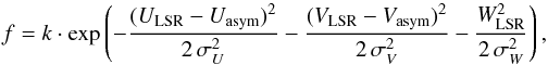 (A.1)where
  (A.2)normalises the expression. σU, σV, and σW are the characteristic velocity dispersions, and Vasym is the asymmetric drift. The values for the velocity dispersions, rotational lags, and normalisations in the Solar neighbourhood that we used are listed in Table A.1.
To get the probability (which we will call D, TD, and H, for the thin disk, thick disk, and stellar halo, respectively) that a given star belongs to a specific population the probabilities from Eq. (A.1) should be multiplied by the observed fractions (X) of each population in the Solar neighbourhood. By then dividing the thick disk probability (TD) with the thin disk (D) and halo (H) probabilities, respectively, we get two relative probabilities for the thick disk-to-thin disk (TD/D) and thick disk-to-halo (TD/H) membership, i.e.  (A.3)and likewise for other probability ratios.
Appendix B: Description of error analysis method
The method is taken from Epstein et al. (2010) and is based on the fact that the four stellar parameters mj = (Teff, ξt, log g, log (Fe)) have been determined using four observables, oi:
-
o1: the first observable is the slope from the linear regression when plotting abundances from Fe i lines versus excitation potential. For the best fit of the effective temperature (Teff) this slope should be zero;
-
o2: the second observable is the slope from the linear regression when plotting abundances from Fe i lines versus reduced line strength (log (W/λ)). For the best fit of the micro-turbulence parameter (ξt) this slope should be zero;
-
o3: the third observable is the abundances from Fe i and Fe ii lines. For a correctly determined surface gravity, they should be equal;
-
o4: the fourth observable is the difference between the output abundance from Fe i lines and the input metallicity of the stellar model that is used. For the best fit this difference should be zero.
Each observable can be written as a linear combination of deviations from the best fit model:  (B.1)where bij = ∂oi/∂mj = Δoi/Δmj are the partial derivatives of the observables. The values for bij are determined by varying each of the stellar parameters one at a time by an amount of Δmj. We choose to set Δm1 = ± 100 K, Δm2 = ± 0.1 km s-1, Δm3 = ± 0.1 dex, and Δm4 = ± 0.1 dex. Applying these changes in the stellar parameters, we then calculate four sets of new abundances for all lines. Compared to the best fit model, we will now see changes in the observables
  (where
  is the value of the observable from the best fit model). Eq. (B.1) gives a system of equations to be solved. Inverting the 4 × 4 matrix of bij gives a new 4 × 4 matrix of elements cik. As each observable oi is associated with an error (σk), the uncertainties in the stellar parameters (mi) can be then solved as:
  (B.2)For o1, which is the slope of the Fe i abundances versus excitation potential that is used for the determination of Teff, we take σ1 as the uncertainty of the linear regression in that plot. For o2, which is the slope of the abundances from Fe i lines versus reduced line strength, we take σ2 as the uncertainty of the linear regression in that plot. For o3, σ3 is connected to the formal errors in the Fe i and Fe ii abundances. σ4, associated with the observable for the balance between input and output abundances, is similar to σ3, but since we only use Fe i lines to measure log (Fe), we use the formal error that we measure for abundances from Fe i lines as σ4. The final estimates of the uncertainties in the stellar parameters, as calculated by Eq. (B.2), are given together with the best fit values of the stellar parameters in Table C.3.
The measured abundance of an element (X) can be written as a linear combination of deviations from the best fit model  (B.3)where the partial derivatives κj = ∂X/∂mj = ΔX/Δmj are calculated for all elements (X) by changing the stellar model atmosphere parameters by the same amounts as when determining bij above, and αj is given by
  (B.4)The error in the measured average abundance for an element then becomes
  (B.5)where σk are the uncertainties in the observables as given above, and σX0 is the formal error of the measured abundance. The uncertainty in a measured abundance ratio [X/Y] is then
 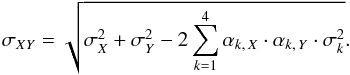 (B.6)Uncertainties in the stellar parameters and in the abundance ratios ([X/Fe] and [X/Ti]) are given in Table C.3 for all 714 stars.
Appendix C: Description of online tables
We are providing three online tables. The first table (Table C.1) lists the stars that were rejected from further analysis. The reasons are given in the table but the main causes are that the stars are either spectroscopic binaries and/or rotated too fast to allow for proper measurements of the equivalent widths. The next table (Table C.2) gives the atomic data and the equivalent widths and elemental abundances for individual lines in the Sun. The third table (Table C.3) gives the results, kinematics, ages, abundance ratios, and uncertainties for the full sample of 714 stars. Details on all three tables are given below.
Stars observed but rejected from analysis.
Atomic line data and measured equivalent widths and absolute abundances in the Sun.
Stellar parameters, ages, abundance ratios, uncertainties, and kinematical properties for the 714 stars.
© ESO, 2014
Current usage metrics show cumulative count of Article Views (full-text article views including HTML views, PDF and ePub downloads, according to the available data) and Abstracts Views on Vision4Press platform.
Data correspond to usage on the plateform after 2015. The current usage metrics is available 48-96 hours after online publication and is updated daily on week days.
Initial download of the metrics may take a while.