| Issue |
A&A
Volume 562, February 2014
|
|
|---|---|---|
| Article Number | A80 | |
| Number of page(s) | 14 | |
| Section | Planets and planetary systems | |
| DOI | https://doi.org/10.1051/0004-6361/201322258 | |
| Published online | 10 February 2014 | |
Online material
Appendix A: Atmospheric model
First, we describe opacity models for the water vapor atmosphere. We define the
Planck-type (κP) and the Rosseland-type mean opacities
(κr) as 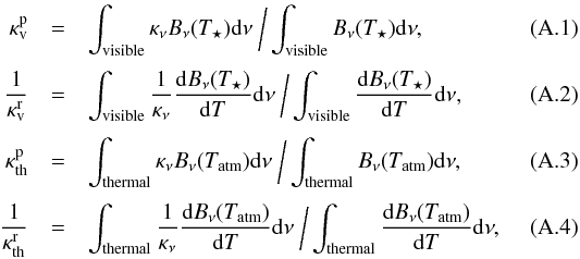 where
ν is the frequency; κν
the monochromatic opacity at a given ν;
T⋆ the stellar effective temperature;
Tatm the atmospheric temperature of the planet; and
Bν the Planck function. The subscripts,
“th” and “v”, mean opacities in the thermal and visible wavelengths, respectively. In
this study, we assume T⋆ = 5780 K. We adopt
HITRAN opacity data for water (Rothman et al.
2009) and calculate mean opacities for 1000 K, 2000 K, and 3000 K at 1, 10, 100
bar. Mean opacities are fitted to power-law functions of P and
T, using the least squares method;
where
ν is the frequency; κν
the monochromatic opacity at a given ν;
T⋆ the stellar effective temperature;
Tatm the atmospheric temperature of the planet; and
Bν the Planck function. The subscripts,
“th” and “v”, mean opacities in the thermal and visible wavelengths, respectively. In
this study, we assume T⋆ = 5780 K. We adopt
HITRAN opacity data for water (Rothman et al.
2009) and calculate mean opacities for 1000 K, 2000 K, and 3000 K at 1, 10, 100
bar. Mean opacities are fitted to power-law functions of P and
T, using the least squares method; 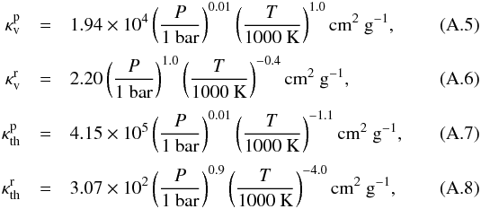 where
P is the pressure and T the temperature.
where
P is the pressure and T the temperature.
In this study, we basically follow the prescription developed by Guillot (2010) except for the treatment of the opacity. We consider a
static, plane-parallel atmosphere in local thermodynamic equilibrium. We assume that the
atmosphere is in radiative equilibrium between an incoming visible flux from the star
and an outgoing infrared flux from the planet. Thus, the radiation energy equation and
radiation momentum equation are written as 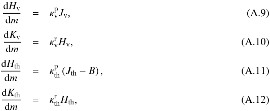 and
the atmosphere in radiative equilibrium satisfies
and
the atmosphere in radiative equilibrium satisfies 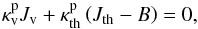 (A.13)where
Jv (Jth),
Hv (Hth), and
Kv (Kth) are, respectively,
the zeroth-, first-, and second-order moments of radiation intensity in the visible
(thermal) wavelengths, m the atmospheric mass coordinate,
dm = ρdz, where z
is the altitude from the bottom of the atmosphere, ρ the density, and
B the frequency-integrated Planck function,
(A.13)where
Jv (Jth),
Hv (Hth), and
Kv (Kth) are, respectively,
the zeroth-, first-, and second-order moments of radiation intensity in the visible
(thermal) wavelengths, m the atmospheric mass coordinate,
dm = ρdz, where z
is the altitude from the bottom of the atmosphere, ρ the density, and
B the frequency-integrated Planck function,
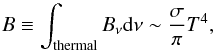 (A.14)where
σ is the Stefan-Boltzmann constant. We assume here that thermal
emission from the atmosphere at visible wavelengths are negligible, so that
Bν ~ 0 in the visible region. The six
moments of the radiation field are defined as
(A.14)where
σ is the Stefan-Boltzmann constant. We assume here that thermal
emission from the atmosphere at visible wavelengths are negligible, so that
Bν ~ 0 in the visible region. The six
moments of the radiation field are defined as 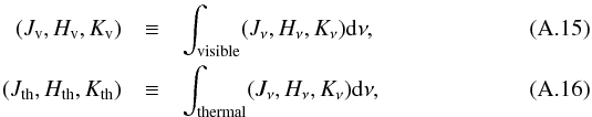 where
Jν is the mean intensity,
4πHν the radiation flux,
and
4πKν/c
the radiation pressure (c is the speed of light).
where
Jν is the mean intensity,
4πHν the radiation flux,
and
4πKν/c
the radiation pressure (c is the speed of light).
We integrate three moments of specific intensity,
Jν,Hν
and Kν, over all the frequencies:
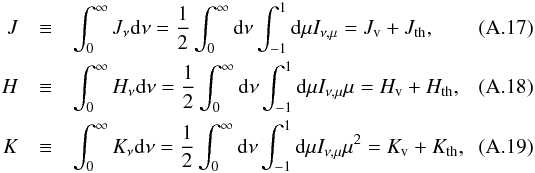 where
Iν,μ is the specific intensity and
θ the angle of a intensity with respect to the
z-axis, μ = cosθ. The energy
conservation of the total flux implies
where
Iν,μ is the specific intensity and
θ the angle of a intensity with respect to the
z-axis, μ = cosθ. The energy
conservation of the total flux implies 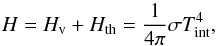 (A.20)where
Tirr is the irradiation temperature given by
(A.20)where
Tirr is the irradiation temperature given by
 (A.21)where
R⋆ is the radius of the host star and
a the semi-major axis.
(A.21)where
R⋆ is the radius of the host star and
a the semi-major axis.
For the closure relations, we use the Eddington approximation (e.g. Chandrasekhar 1960), namely,
 For
an isotropic case of both the incoming and outgoing radiation fields, we find boundary
conditions of the moment equations as follows (see also Guillot 2010, for details):
For
an isotropic case of both the incoming and outgoing radiation fields, we find boundary
conditions of the moment equations as follows (see also Guillot 2010, for details):  Thus,
we integrate Eqs. (A.9)–(A.13) over m numerically,
using mean opacities of (A.5)–(A.8) and boundary conditions of (A.24)–(A.26), and then determine a T–P
profile of the water vapor atmosphere. We assume that the boundary is at
P0 = 1 × 10⁻⁵ bar. The choice of
P0 (≤1 × 10⁻⁵bar) has little effect on the
atmospheric temperature-pressure structure. T0 is determined
in an iterative fashion until
abs(T0 − [πB(m = 0,P0,T0)/σ] 1/4) ≤ 0.01
is fulfilled. Then we integrate Eqs. (A.9)–(A.13) over
m by the 4th-order Runge-Kutta method, until we find the point where
dlnT/dlnP ≥ ∇ad. The
pressure and temperature, Pad and
Tad, are the boundary conditions for the
convective-interior structure (see Sect. 2.1).
Thus,
we integrate Eqs. (A.9)–(A.13) over m numerically,
using mean opacities of (A.5)–(A.8) and boundary conditions of (A.24)–(A.26), and then determine a T–P
profile of the water vapor atmosphere. We assume that the boundary is at
P0 = 1 × 10⁻⁵ bar. The choice of
P0 (≤1 × 10⁻⁵bar) has little effect on the
atmospheric temperature-pressure structure. T0 is determined
in an iterative fashion until
abs(T0 − [πB(m = 0,P0,T0)/σ] 1/4) ≤ 0.01
is fulfilled. Then we integrate Eqs. (A.9)–(A.13) over
m by the 4th-order Runge-Kutta method, until we find the point where
dlnT/dlnP ≥ ∇ad. The
pressure and temperature, Pad and
Tad, are the boundary conditions for the
convective-interior structure (see Sect. 2.1).
In Fig. A.1, we show the
P–T profile for the solar-composition atmosphere
with g = 980 cm s-2, Tint = 300
K, and Tirr = 1500 K (dotted line). In this calculation, we
take  and
and
 as functions of
P and T from Freedman
et al. (2008) and calculate
as functions of
P and T from Freedman
et al. (2008) and calculate  and
and
 , for
P = 1 × 10-3,0.1,1,10
bar and T = 1500 K from HITRAN and HITEMP data that include
H2, He, H2O, CO, CH4, Na, and K for the solar
abundance respectively as
, for
P = 1 × 10-3,0.1,1,10
bar and T = 1500 K from HITRAN and HITEMP data that include
H2, He, H2O, CO, CH4, Na, and K for the solar
abundance respectively as 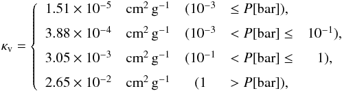 (A.27)by
use of (A.2). The thin and thick parts
of the dotted line represent the radiative and convective zones, respectively.
(A.27)by
use of (A.2). The thin and thick parts
of the dotted line represent the radiative and convective zones, respectively.
In addition, we test our atmosphere model by comparing it with the P–T profile derived by Guillot (2010) with γ = κv/κth = 0.4 (solid line), which reproduces more detailed atmosphere models by Fortney et al. (2005) and Iro et al. (2005, see Fig. 6 of Guillot 2010). As seen in Fig. A.1, our atmospheric model yields a P–T profile similar to that from Guillot (2010). In our model, temperatures are relatively low compared with the Guillot (2010) model at P ≲ 40 bar, which is due to difference in opacity. In our model, deep regions of P ≳ 40 bar are convective, while there is no convective region in the Guillot (2010) model because of constant opacity. We have compared our P–T profile with the Fortney et al. (2005)’s and Iro et al. (2005)’s profiles, which are shown in Fig. 6 of Guillot (2010) and confirmed that our P–T profile in the convective region is almost equal to their profiles. Of special interest in this study is the entropy at the radiative/convective boundary, because it governs the thermal evolution of the planet. In this sense, it is fair to say that our atmospheric model yields appropriate boundary conditions for the structure of the convective interior.
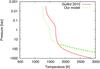 |
Fig. A.1
Temperature–pressure profiles for a solar-composition atmosphere (see the details in text). The solid (red) and dotted (green) lines represent both Guillot (2010)’s (γ = 0.4) and our model’s, respectively. The thin and thick parts of the dotted line represent the radiative and convective regions, respectively. We have assumed g = 980 cm s-2, Tint = 300 K, and Tirr = 1500 K. |
| Open with DEXTER | |
Finally, we describe an analytical expression for our atmospheric model. We basically
follow the prescription developed by Heng et al.
(2012), except for the treatment of the opacity. As Heng et al. (2012) mentioned, it would be a challenging task without
assumption of constant  and
and
 to obtain
analytical solutions for Jv and
Hv. Here we assume and
are
constant throughout the atmosphere. We differentiate (A.9) and (A.10) by
m and obtain
to obtain
analytical solutions for Jv and
Hv. Here we assume and
are
constant throughout the atmosphere. We differentiate (A.9) and (A.10) by
m and obtain 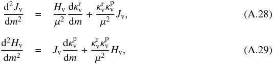 where
μ2 = Kv/Jv.
Assuming Jv = Hv = 0 as
m → ∞, we obtain
where
μ2 = Kv/Jv.
Assuming Jv = Hv = 0 as
m → ∞, we obtain
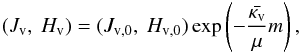 (A.30)where
 and Jv,0 and
Hv,0 are the values of
Jv and Hv evaluated at
m = 0, respectively. In general, the heat transportation, such as
circulation, produces a specific luminosity of heat. Heng et al. (2012) introduced the specific luminosity as Q,
which has units of erg s-1 g-1. Q can be related
to the moments of the specific intensity and we obtain
and Jv,0 and
Hv,0 are the values of
Jv and Hv evaluated at
m = 0, respectively. In general, the heat transportation, such as
circulation, produces a specific luminosity of heat. Heng et al. (2012) introduced the specific luminosity as Q,
which has units of erg s-1 g-1. Q can be related
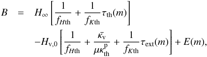
to the moments of the specific intensity and we obtain 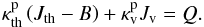 (A.31)We integrate Eq. (A.31) and obtain
  (A.32)where
H∞ is the value of H evaluated at
m → ∞ and
(A.32)where
H∞ is the value of H evaluated at
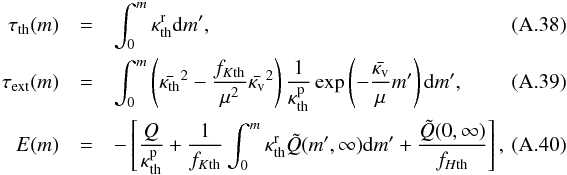
m → ∞ and 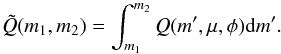 (A.33)To obtain
Hth and Jth, we substitute Eq.
(A.31) in Eqs. (A.11) and (A.12) and integrate by m. Then we obtain
(A.33)To obtain
Hth and Jth, we substitute Eq.
(A.31) in Eqs. (A.11) and (A.12) and integrate by m. Then we obtain
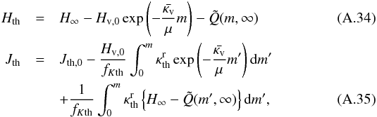 where
fKth = Kth/Jth,
fHth = Hth/Jth,
and
where
fKth = Kth/Jth,
fHth = Hth/Jth,
and 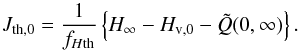 (A.36)That is, we obtain
 (A.37)where
 and
and
 .
In our conditions, we assume
.
In our conditions, we assume  ,
fKth = 1/3,
fHth = 1/2 and
Q = 0. Consequently, we obtain
,
fKth = 1/3,
fHth = 1/2 and
Q = 0. Consequently, we obtain
the temperature profile as 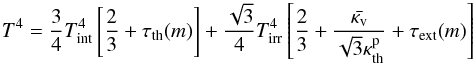 (A.41)where
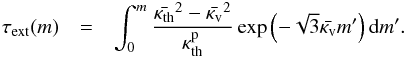 (A.42)If
we assume
(A.42)If
we assume  and
and
 , Eq. (A.41) agrees with Eq. (27) of Heng et al. (2012).
© ESO, 2014
Current usage metrics show cumulative count of Article Views (full-text article views including HTML views, PDF and ePub downloads, according to the available data) and Abstracts Views on Vision4Press platform.
Data correspond to usage on the plateform after 2015. The current usage metrics is available 48-96 hours after online publication and is updated daily on week days.
Initial download of the metrics may take a while.