| Issue |
A&A
Volume 561, January 2014
|
|
|---|---|---|
| Article Number | A125 | |
| Number of page(s) | 22 | |
| Section | Stellar structure and evolution | |
| DOI | https://doi.org/10.1051/0004-6361/201322210 | |
| Published online | 21 January 2014 | |
Online material
Appendix A: Kernel density and LOWESS
The kernel density is a non-parametric estimate of the probability density function from a discrete set of data. It can be viewed as a generalization of the histogram, with better theoretical properties (Härdle & Simar 2012). For a set of n observations x1, x2, ..., xn, a kernel density with bandwidth h has the form: 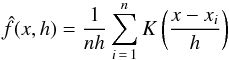 (A.1)where the kernel function K is chosen to be a probability density function. Several choices of kernel are available. In this work. we make use of a Gaussian kernel:
 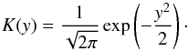 (A.2)The kernel selection usually has a minor influence on the kernel estimate with respect to the bandwidth h. This parameter is selected balancing two effects since an increment of h increases the bias of
  , while it reduces its variance. An often adopted choice for a Gaussian kernel is given by the rule of thumb (Silverman 1986):
 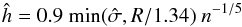 (A.3)where
  is the sample standard deviation and R the sample interquartile range.
Other choices for the bandwidth, based on the asymptotic expansion of the mean integrated squared error, are reported in the literature. The different choices have an impact on kernel estimator for multi-modal distributions, which is not the case of the present work. We refer interested readers to Feigelson & Babu (2012), Härdle & Simar (2012), Venables & Ripley (2002), Sheather & Jones (1991).
A frequently used bivariate smoother is the local regression technique LOWESS, which combines a linear least squares regression with a robust nonlinear regression. It provides a generally smooth curve, whose value at a particular location along the x axis is only determined by the points in its neighbourhood. The first step is to fit a polynomial regression in a neighbourhood of x. A fraction f of the n sample points near x is selected. We define m = ⌈ fn ⌉ the number of points used in the fit. Then the technique obtains the estimates  by minimizing
 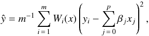 (A.4)where Wi(x) are the weights, usually obtained by the tricubic function:
 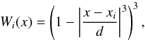 (A.5)where d is the maximum distance between x and the other predictor values xi in the span. For LOWESS estimates the value p = 1 is usually adopted, implying a local linear regression. The model residuals
  and the scale parameter
  are computed. The median absolute deviation of the residuals is evaluated:
  . Then the algorithm computes the robustness weights
  , with R(u) = 15/16(1 − u)2 for | u | ≤ 1 and R(u) = 0 otherwise. The local regression of Eq. (A.4) is computed again, but with weights given by δiKi(x). This procedure is iterated a variable number of times between one and five; this makes the local estimate robust even in presence of outliers. Further details on the technique and on the numerical methods used to speed up the computations are available in Cleveland (1981).
The computations outlined in this section were performed using the functions density and lowess, available in the R 2.15.2 (R Development Core Team 2012).
Summary of mass and radius relative errors.
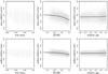 |
Fig. 6
As in Fig. 2, but for data sampled from a grid with ΔY/ΔZ = 1, and recovered with the standard grid adopting ΔY/ΔZ = 2. |
| Open with DEXTER | |
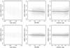 |
Fig. 8
As in Fig. 2, but for synthetic data sampled from a grid with αml = 1.50, and estimated with the standard grid (i.e. αml = 1.74). |
| Open with DEXTER | |
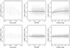 |
Fig. 9
As in Fig. 2, but for synthetic data sampled from a grid with αml = 1.98 and estimated with the standard grid (i.e. αml = 1.74). |
| Open with DEXTER | |
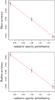 |
Fig. 10
As in Fig. 5, but for synthetic data sampled from grids with different values of radiative opacity and reconstructed with the standard grid. |
| Open with DEXTER | |
 |
Fig. 11
As in Fig. 2, but for synthetic data sampled from a grid with kr at its low value, estimated on the standard grid. |
| Open with DEXTER | |
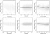 |
Fig. 13
As in Fig. 2, but for synthetic data sampled from the standard grid and recovered on the grid, which does not include diffusion in the computations. |
| Open with DEXTER | |
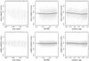 |
Fig. 14
As in Fig. 2, but for synthetic data sampled from the standard grid and recovered on the same grid but without taking the surface [Fe/H] evolution into account. |
| Open with DEXTER | |
© ESO, 2014
Current usage metrics show cumulative count of Article Views (full-text article views including HTML views, PDF and ePub downloads, according to the available data) and Abstracts Views on Vision4Press platform.
Data correspond to usage on the plateform after 2015. The current usage metrics is available 48-96 hours after online publication and is updated daily on week days.
Initial download of the metrics may take a while.