| Issue |
A&A
Volume 560, December 2013
|
|
|---|---|---|
| Article Number | A24 | |
| Number of page(s) | 25 | |
| Section | Interstellar and circumstellar matter | |
| DOI | https://doi.org/10.1051/0004-6361/201321592 | |
| Published online | 29 November 2013 | |
Online material
Appendix A: Noise maps
We create noise maps from both the 13CO (2–1) and the C18O (2–1) data cubes. For each spectrum, we determine the root-mean-square (rms) and create maps from these values. For this purpose, we need to calculate the rms from parts of the spectra that are emission-free. We use the velocity range between 120 and 130 km s-1, because it is free of emission for the complete region that we mapped. Typical values are found to be around 1 K or even less, while some parts in the south show values of up to 3 K. All values given here are in Tmb, which are corrected for main beam efficiency. The results can be seen in Fig. A.1.
We find that the structure of the noise is similar for both lines. The largest differences arise from weather conditions and time of day. This is seen in the squarish pattern, as each square shows single observations that have been carried out in a small time window. Still, there is a striped pattern visible that overlays the whole map. This stems from the nine different pixels that make up the HERA receiver. These pixels have different receiver temperatures, hence the different noise levels. We also note that observations in the northern part of the map are usually less noisy than those in the south. This probably results from the different weather in which the observations have been carried out. Last, we find that the C18O (mean rms of 1.3 K, maximum of 6.7 K) data shows a little increase in noise temperature in general compared to the 13CO line (mean rms of 1.1 K, maximum of 3.7 K). The latter has been observed with the HERA1 polarization of the HERA receiver, whereas the first has been observed with HERA2, which has an overall higher receiver temperature.
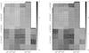 |
Fig. A.1
Noise level maps in Tmb with scale in [K]. Left: 13CO (2–1) map. Right: C18O (2–1) map. |
| Open with DEXTER | |
Appendix B: Peak velocity and line width of foreground components
Figure B.1 shows plots of the peak velocity position and the FWHM line width of the two lower velocity components. The maps of the W43 complex itself are shown in Fig. 7 and are described in Sect. 3.4.
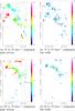 |
Fig. B.1
Maps of the first (line peak velocity) and second (line width FWHM) moment maps of the two fore-/background components. |
| Open with DEXTER | |
Appendix C: Calculations
Appendix C.1: 13CO optical depth
Assuming a constant abundance ratio of 12CO:13CO:C18O, we can estimate the optical depth of the 13CO gas (see e.g. Myers et al. 1983; Ladd et al. 1998). We compare the intensities of the 13CO and C18O line emission integrated over the analyzed cloud and solve the equation, 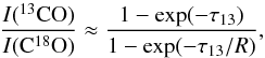 (C.1)for τ13, where R is the intrinsic ratio of the two mapped CO isotopologes.
The isotopic abundance of C and O in the Milky Way is known to depend on the Galactocentric radius. Often cited values are found in Wilson & Rood (1994). They find the ratio of 16O and 18O to be 272 at 4 kpc radius, 302 at 4.5 kpc, and 390 at 6 kpc, so we take those numbers for the 12CO:C18O ratio. Recent values for the C/13C abundance are given in Milam et al. (2005). Here, we take values derived from CO observations and get a 12CO:13CO ratio of 31 at a Galactocentric radius of 4 kpc for the main component and a ratio of 43 and 52 for the foreground components at a radius of 4.5 and 6 kpc, respectively. In total, we use an intrinsic ratio of 12CO:13CO:C18O of 1:1/31:1/272 for sources in the main complex and ratios of 1:1/43:1/302 and 1:1/52:1/390 respectively for foreground sources.
Appendix C.2: Excitation temperature
Once we know the optical depth, we can determine the excitation temperature of the CO gas.
For this, we use Ladd et al. (1998): 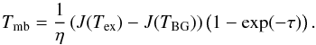 (C.2)With
  (C.3)we use the line peak intensity Tpeak for Tmb. The parameter TBG is the cosmic background radiation of 2.7 K, τ the 13CO optical depth, and η the beam filling factor. This expression can then be solved for Tex.
Here, we assume that the excitation temperature of 13CO and C18O is the same. We then assume that the beam filling factor η is always 1. It is likely that there is some substructure that we cannot resolve with our beam size. This would mean that the real η is lower than 1, and we calculate Tex × η rather than just Tex. Thus, we underestimate the temperature in cases where there is indeed substructure. The line peak Tpeak is calculated from fitting a Gaussian to all spectra in the 13CO line emission cube.
We cannot calculate a Tex in this way for all pixels, even if 13CO is present, as the C18O is much weaker. As the ratio of 13CO and C18O is needed, a self-consistent temperature can only be computed for points where C18O is present. The main uncertainty of the calculation itself is the assumption that the beam filling factor is always 1, and the real value can only be correctly derived where this is true. This led to the decision not to use these Tex maps for the further calculation of the H2 column density. We used the calculations to get an idea of the gas temperature and then used a constant value for all further steps of analysis. We chose this value to be 12 K, as this was the median temperature found across the whole W43 region.
Appendix C.3: Column density and mass
We then compute the H2 column density by using the assumed excitation temperature Tex of 12 K and the integrated molecular line emission from our observation through  (C.4)where the factor containing τ accounts for the effect that the full gas is not seen for optically thicker clouds and
  (C.5)with the function
  (C.6)where B = 5.5099671 × 10¹⁰ s-1 is the rotational constant for 13CO, μ = 0.112 D is its dipole moment, and Ju is the upper level of our transition (2 in this case). We correct all those points for the optical depth where we find an opacity larger than 0.5. We assume this is the minimum value we can determine correctly as we might confuse emission with noise for lower opacities.
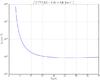 |
Fig. C.1
13CO column density depending on the excitation temperature. |
| Open with DEXTER | |
In Fig. C.1 we plot the dependency of the 13CO column density and the excitation temperature. We note that the column density for values of >15 K is nearly independent of the excitation temperature. On the contrary, it rises steeply for temperatures below 10 K. This is important as we most probably would underestimate the excitation temperature for most clouds as discussed above, if we actually used the calculated Tex. We would thus overestimate the column density. Therefore, we can assume that using an excitation temperature of 12 K for our calculation results in a lower limit for the actual column density.
As we want to calculate the H2 column density, we need to translate N(13CO) into N(H2). The standard factor of N(H2):N(12CO) is 104 for local molecular clouds, but the ratio varies with sources and also with the Galactocentric radius. Fontani et al. (2012) derives a radius dependent formula for N(H2):N(CO), using values of 12C/H and 16O/H from Wilson & Matteucci (1992). This formula gives a ratio of 6550 for a Galactic radius of 4 kpc 7000 at 4.5 kpc and 8500 at 6 kpc. Using our ratios of 12CO:13CO from above we get N(H2) = 2.0 × 10⁵ N(13CO) for the W43 complex with a radius of 4 kpc and the factors of 3.0 × 10⁵ and 4.4 × 10⁵ for the fore-/background complexes with radii of 4.5 and 6 kpc components, respectively. These factors are prone to large errors of at least a factor of 2.
To calculate the mass of the observed source from the H2 column density it is necessary to consider the relative distance from the Sun to the source. See Sect. 3.3 for the distance determination. We assume the main complex clouds are 6 kpc away, while the foreground clouds have distances of 3.5, 4, 3.5, and 12 kpc. Then, we just have to count the number of H2 molecules per pixel to receive the mass per pixel in solar masses. 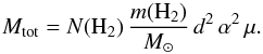 (C.7)Here, d is the distance toward the source, α the angular extent of one pixel on the sky. The value of μ = 1.36 accounts for higher masses of molecules, apart from H2 (compare Schneider et al. 2010).
The resulting H2 column density map of the full W43 complex is shown in Fig. 10, which was calculated using the velocity range between 78 and 120 km s-1. It has been calculated for all points, where the integrated 13CO shows an intensity of more than 5 K km s-1. The integrated 13CO map in Fig. 1a shows diffuse emission in-between the brighter sources that were isolated with the Duchamp sourcefinder. This diffuse emission accounts for about 50% of the the total mass in W43.
Appendix D: Description of important sources
In the following, we want to give a description of several important and interesting sources of the W43 complex (d = 6 kpc) found in our datasets. Information on these sources are listed in Table 1, while their location is indicated in Fig. 4. The corresponding maps can be found in Fig. E.1. We discuss the shape, topology, and intensity of the maps and fundamental properties like velocity gradients, FWHM line widths, temperature, and column density. We also mention conclusions from the comparison to different datasets. Sources are ordered by their peak velocities.
Appendix D.1: Source 23
Source 23 (plots can be seen in Fig. 11 and also Fig. E.1w) consists of one central elliptical clump with one elongated thin extension, protruding from the southeast, that ends in a hook-like tip and is curved to the south. The central clump is elliptically shaped with a length of 5 and 3 parsec on the major axes and is bound sharply at the southern edge, while it is much more diffuse and more extended in the north. The extension has a length of 7.5 pc. We find the maximum integrated intensity of the 13CO (2–1) line to be about 90 K km s-1 at the peak of the clump, while the filamentary extension lies around 30 to 45 K km s-1. The line peak intensity rises from 12 K in the filament to 24 K in the clump. The opacity has typical values of 1 to 2.5 with higher values in the central clump.
We see a gradient in the radial velocity of the cloud from the filament to the center of the source of ~ 3 km s-1, which can be interpreted as a flow of gas along the outrigger onto the clump. The line width (FWHM) changes between 4.5 km s-1 in the inner clump and 2 to 2.5 km s-1 in the outer parts of the cloud.
The H2 column density that we calculated rises from ~ 5 × 1021 cm-2 in the edges of the cloud to ~ 7 × 1022 cm-2 in the center. The total mass is calculated to be 2.7 × 10⁴M⊙ and thus resembles a typical total mass of our set of sources.
The CO emission that we measure in our maps is nearly exactly matched by the dust emission maps of ATLASGAL and Hi-GAL (see Figs. 11b and c, respectively). Both show the strong peak in the central clump and the weaker filament in the southeast, including that of the curved tip. The GLIMPSE map shows very interesting features (see Fig. 11d). There is one strong UV point source less than 1 pc off to the south of the CO clump.
Appendix D.2: Source 25
This filament, as seen in Fig. E.1y, resides in the central western part of the W43 complex, which is half-way between W43-Main and W43-South. It is shaped like an inverted L with two branches and connected by an orthogonal angle. The vertical branch has a length of 14 pc; the horizontal one is 10 pc long. The typical width of both branches is between 2 and 3 pc. One strong clump is seen in the southern part with an integrated line intensity of the 13CO (2–1) line of 40 K km s-1, while the rest of the filament backbone only reaches 18 to 22 K km s-1. Line peak intensities range from a few K in the outer parts of the filament up to 15 K in the strong southern clump.
Investigating the line peak velocity map, we realize that the two branches of this source are actually separated. The horizontal branch has a constant radial velocity of 108 km s-1 across, while the vertical branch shows a gradient from 110 km s-1 in the north to 115 km s-1 in the south. Line widths range between 1 and 2 km s-1 in the whole source.
The H2 column density varies between 2 × 1021 cm-2 in the outer parts and 4 × 1022 cm-2 around the southern core. The total mass is ~ 6.8 × 10³M⊙. Comparing this source to the complementary projects is complicated, since the source 17 is located at the same place and overlaps this source. Most emission that is seen in the northern part of the source is presumably part of source 17. Only the embedded core in the south is clearly seen in dust emission and as a compact Spitzer source.
Appendix D.3: Source 26
Located in the easternmost central part of the W43 complex lies this filamentary shaped source, whose plot is found in Fig. E.1z. It stretches over a range of 26 pc from southeast to northwest. The filament consists of three subsections that contain several clumps and has a typical width of 5 pc. The integrated emission map of the 13CO (2–1) line shows values of up to 35 K km s-1 in the clumps, which is surrounded by weaker gas. The strongest clump lies in the southeastern end of the filament while the highest line peak intensities are found in the northwest with up to 13 K.
The velocity structure of this filament is nearly symmetrical, starting around 106 km s-1 in the middle of the filament and increasing toward its tips up to 110 km s-1 in the west and 112 km s-1 in the east. The width of the lines has nearly homogeneous values around 2 km s-1 in the center and western part of the filament but shows broad lines with a width of more than 5 km s-1 in the eastern clump.
This filament shows a typical distribution of its H2 column density. Several denser clumps are embedded along the filament. Column densities vary from a few 1021 cm-2 in the outer parts of the filament up to a maximum of 3 × 1022 cm-2 in one clump. The total mass of this source is 1.7 × 10⁴M⊙.
The CO emission of this source matches nicely with the dust emission of ALTASGAL and Hi-GAL. However, the eastern part of the filament is stronger in the 850 μm map than the shorter wavelengths of Hi-GAL and vice versa in the western part. Only the clump in the west of this filament can be seen in the 8 μm Spitzer data, the east is not traced. There is one extended source seen in emission in the center part of this source, but this is probably unrelated.
Appendix D.4: Source 28
Source 28 (see Fig. E.1a, b) is located in the southwest of W43-Main in the central region of the complex. It is not visible in the total integrated maps of the region, as it is confused with sources of a different relative velocity. It becomes visible by investigating the channel maps between 110 and 115 km s-1 radial velocity. The source has dimensions of 12 pc in the east-west direction and 8 pc in the north-south direction. Its shape is that of a two-armed filament, whose two parts join at an angle of ~ 135° where the eastern arm runs from southeast to northwest and the western arm from east to west. We see two stronger clumps in the eastern filament: one in the center of it and one in the southeastern tip. This is a relatively weak source with an integrated 13CO (2–1) emission that peaks at only 25 K km s-1 in the center of the eastern filament, where the maximum line peak is around 13 K. The integrated intensity goes down to 8 K km s-1 in the outskirts of the filament. Yet, it is a valuable source, due to its pronounced filamentary structure and the embedded clumps, which is a good candidate for more investigations in filament formation (see Carlhoff et al., in prep., for additional observations and analysis of this cloud).
The eastern arm is especially interesting. It has a length of 6 pc and a typical width of 1.5 pc. We note two embedded clumps embedded in it and a velocity gradient along the filament, which starts at 110 km s-1 in the north and increases to 114 km s-1 in the southeastern part of this arm. The typical line width varies between 1 and 2 km s-1, increasing toward the inside of the cloud and reaching the maximum width at the clumps.
As this source is rather weak, we also find H2 column densities to be only around 2 × 1022 cm-2 at the maximum around the embedded clumps. The total derived mass of the molecular gas is ~ 4300 M⊙, which makes it one of the less massive sources identified.
Surprisingly, this source is one of the few that is not traced at all in the GLIMPSE 8 μm map. It appears that there are no nearby UV sources that could heat the gas. The two nearest sources were identified to be related to background sources in another Galactic spiral arm. Also, the gas and the related dust is obviously too faint to appear in absorption. This is also verified by the ATLASGAL an Hi-GAL maps, which show only weak dust emission in the filament.
Appendix D.5: Source 29
This source is found in the very center of our region maps, directly south of the W43-Main cloud. Its shape resembles a
crescent moon, opened toward the southeast, where it is sharply bound. The outside is more diffuse and shows several outflows away from the center. See Fig. E.1a, c for a plot of the 13CO emission. The extent of the source is 12 pc from northeast to southwest, and the filament has a typical width of 2 to 3 pc. Two stronger clumps with an integrated 13CO intensity of 40 K km s-1 are seen in the center and the northeastern tip. The strong backbone of this source has still an integrated intensity of ~ 20 K km s-1, where line peak intensity goes up to 18 K.
The central western part of the source moves with a relative radial velocity of 112 km s-1 and increases to 118 km s-1 toward both ends of the crescent. The lines show widths of 2 to 3 km s-1 in the central region, decreasing to 1 km s-1 in the outer parts. H2 column densities only reach a few 1022 cm-2 across the inner parts of the structure. We find a total mass of 1.2 × 10⁴M⊙.
In the dust emission maps of ATLASGAL and Hi-GAL, only the strong backbone of this source can be seen. The weaker outliers are not traced. The Spitzer 8 μm map shows several bright compact sources in the center, and some extended emission in the south is most probably related to this source. However, the northern tip that shows strong CO emission is not traced by Spitzer at all.
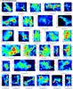 |
Fig. E.1
Integrated 13CO (2–1) maps in K km s-1 of all identified sources. The plots are not proportional to their physical size, as source sizes differ strongly. |
| Open with DEXTER | |
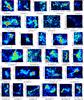 |
Fig. E.2
Integrated C18O (2–1) maps in K km s-1 of all identified sources. |
| Open with DEXTER | |
© ESO, 2013
Current usage metrics show cumulative count of Article Views (full-text article views including HTML views, PDF and ePub downloads, according to the available data) and Abstracts Views on Vision4Press platform.
Data correspond to usage on the plateform after 2015. The current usage metrics is available 48-96 hours after online publication and is updated daily on week days.
Initial download of the metrics may take a while.