| Issue |
A&A
Volume 557, September 2013
|
|
|---|---|---|
| Article Number | A26 | |
| Number of page(s) | 30 | |
| Section | Stellar atmospheres | |
| DOI | https://doi.org/10.1051/0004-6361/201321274 | |
| Published online | 15 August 2013 | |
Online material
Appendix A: The Stagger-grid 1D atmospheres
The following discussion concerns solely 1D atmosphere models and MLT, therefore, similar quantities as discussed above may deviate (e.g. Fconv). The numerical code that we used for computing 1D atmospheres for the Stagger-grid models solves the coupled equations of hydrostatic equilibrium and energy flux conservation in 1D plane-parallel geometry. The 1D models use the same EOS and opacity package in order to allow consistent 3D-1D comparisons. The set of equations and numerical methods employed for their solution are similar to those of the MARCS code (Gustafsson et al. 2008) with a few changes and simplifications that will be outlined in the following. The resulting model atmospheres yet maintain very good agreement with MARCS models (see Sect. 3.3.2).
Appendix A.1: Basic equations
Assuming 1D plane-parallel geometry with horizontal homogeneity and dominance of hydrostatic equilibrium over all vertical flow simplifies the equation of motion (Eq. (2)) to the hydrostatic equilibrium equation  (A.1)where κstd and τstd are a standard opacity and corresponding optical depth (e.g. the Rosseland mean), pgas and pturb denote gas pressure and turbulent pressure, ρ is the gas density, and g is the surface gravity. Radiation pressure is neglected, as in the 3D simulations. Turbulent pressure is estimated using the expression
  (A.2)with the scaling parameter β that corrects for asymmetries in the velocity distribution and the mean turbulent velocity vturb that is used as a free, independent parameter.
The depth-integral of the energy equation (Eq. (3)) reduces to the flux conservation equation,  (A.3)where Frad is the radiative energy flux, Fconv is the convective energy flux, σ is the Stefan-Boltzmann constant and Teff is the stellar effective temperature. Contrary to the 3D case, effective temperature now appears as a boundary value and is thus a free parameter. Owing to numerical instabilities of the formulation, Eq. (A.3) is replaced in the higher atmosphere (τRoss ≲ 10-2) with the radiative equilibrium condition
  (A.4)where Jλ and Sλ are the mean intensity and the source function, similar to Eq. (6). In the 3D case, qrad is explicitly calculated and is nonzero in general. Enforcing the condition of radiative equilibrium qrad ≡ 0 in 1D leads to an atmospheric stratification where an exact balance of radiative heating and cooling in each layer is achieved, ignoring the effects of gas motion.
The mean intensity and the radiative energy flux at each depth are obtained by solving the radiative transfer equation, 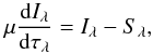 (A.5)where μ = cosθ with the polar angle θ off the vertical, Iλ is the specific intensity at wavelength λ, and τλ is the vertical monochromatic optical depth (with τλ = 0 above the top of the atmosphere). A Planck source function Sλ = Bλ is assumed. The monochromatic mean intensity and radiative flux are then delivered by the integrals
 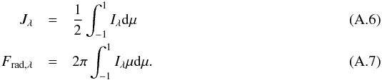 In the absence of an explicit convection treatment, convective energy transfer is estimated using a variant of the mixing length recipe described in Henyey et al. (1965). The convective flux is given by the expression
 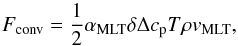 (A.8)where ρ is the gas density, cp is the specific heat capacity, T is the temperature, and vMLT is the convective velocity. The well-known free mixing length parameter αMLT = lm/Hp sets the distance lm in units of the local pressure scale height Hp over which energy is transported convectively. See Gustafsson et al. (2008) for details of the expressions used to obtain the convective velocity vMLT and the factor δΔ = Γ/(1 + Γ)∇sad, which scales super-adiabaticity ∇sad = ∇ − ∇ad of the atmospheric stratification (see also Sect. 3.2.7), by a convective efficiency factor
 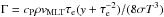 with the optical thickness τe = κRosslm. We adopt the same parameters y = 0.076 and ν = 8 as Gustafsson et al. (2008) for the radiative heat loss term and turbulent viscosity that enter the above quantities.
Appendix A.2: Numerical methods
The system of equations is solved using a modified Newton-Raphson method with an initial stratification of temperature T and gas pressure pgas on a fixed Rosseland optical depth grid. Discretized and linearized versions of the hydrostatic equation and the energy flux equation (or radiative equilibrium condition, respectively) provide the inhomogeneous term and the elements of the Jacobian matrix for the system of 2N linear equations, where N is the number of depth layers. The radiation field is computed for each Newton-Raphson iteration using the integral method, based on a second-order discretization of the fundamental solution of the radiative transfer equation (Eq. (A.5)).
The corrections ΔT and Δpgas derived from the system of linear equations are multiplied by a variable factor < 1 that is automatically regulated by the code to aid convergence. Convergence is assumed when the (relative) residuals of the 2N equations decrease beneath a preset threshold. Note that, contrary to the 3D simulations, the effective temperature is now an adjustable parameter; the requirement of minimal residuals automatically leads to an atmospheric stratification with correct Teff through the energy flux equation.
In order to obtain a 1D model, a given ⟨3D⟩ stratification provides the initial input for the Newton-Raphson iterations, along with the targeted effective temperature and surface gravity. The same EOS tables that were used for the 3D simulation provide gas density, specific heat capacity, and adiabatic gradient as a function of T and pgas. Likewise, the tables containing group mean opacities and the Rosseland mean opacity provide the required microphysics for solving the radiative transfer equation, ensuring maximal consistency with the 3D simulations.
Once convergence has been achieved for the 1D stratification, the mixing length parameter αMLT can be calibrated to obtain a better approximation to the ⟨3D⟩ stratification in the convection zone beneath the stellar surface.
Appendix B: Functional fits
The resulting amount of data from our numerical simulations is enormous. A convenient way to provide important key values is in form of functional fits, which can be easily utilized elsewhere (e.g. for analytical considerations). In the present paper we have frequently discussed various important global properties that are reduced to scalars. Some of them are global scalar values and
some are determined at a specific height from the ⟨3D⟩ stratifications, i.e. temporal and spatial averages on layers of constant Rosseland optical depth. We fitted these scalars with stellar parameters for individual suitable functions, thereby enforcing a smooth rendering. However, we would like to warn against extrapolating these fits outside their range of validity, i.e. outside the confines of our grid. Also, one should consider that possible small irregularities between the grid steps might be neglected, which arise due to non-linear response of the EOS and the opacity. On the other hand, we provide also most of the actual shown values in Table C.1.
We use three different functional bases for our fits and we perform the least-squares minimization with an automated Levenberg-Marquardt method. Instead of the actual stellar parameters, we employ the following transformed coordinates: x = (Teff − 5777)/1000, y = log g − 4.44 and z = [Fe/H]. Furthermore, we find that in order to accomplish an optimal fit with three independent variables, fi(x,y,z), simultaneously, the metallicity should be best included implicitly as nested functions in the form of second degree polynomial  , each resulting in three independent coefficients ai. The linear function
  (B.1)is applied for the following quantities: smin (Fig. 5), log ρpeak (Fig. 18),
  (Fig. 18), log dgran (Fig. 10), log Δtgran and
  . The resulting coefficients are given in Table B.1. On the other hand, we considered the exponential function
  (B.2)for sbot, Δs (Figs. 5 and 18) and [pturb/ptot]peak (Fig. 21). For ∇peak and
  15 we applied the following function
  (B.3)with coefficients for f2 and f3 listed in Table B.2. Finally, we showed in Fig. 7 the entropy jump Δs as a function of sbot, which we fitted with
  (B.4)The resulting coefficients are listed in Table B.3.
Appendix C: Tables
In Table C.1 we have listed important global properties with the stellar parameters. Due to the lack of space, we show only an excerpt with solar metallicity ([Fe/H] = 0.0). The complete table is available at CDS http://cds.u-strasbg.fr.
Stellar parameters: effective temperature, surface gravity (Cols. 1 and 2 in [K] and [dex]).
© ESO, 2013
Current usage metrics show cumulative count of Article Views (full-text article views including HTML views, PDF and ePub downloads, according to the available data) and Abstracts Views on Vision4Press platform.
Data correspond to usage on the plateform after 2015. The current usage metrics is available 48-96 hours after online publication and is updated daily on week days.
Initial download of the metrics may take a while.