| Issue |
A&A
Volume 556, August 2013
|
|
|---|---|---|
| Article Number | A5 | |
| Number of page(s) | 13 | |
| Section | Cosmology (including clusters of galaxies) | |
| DOI | https://doi.org/10.1051/0004-6361/201321172 | |
| Published online | 16 July 2013 | |
Online material
Appendix A: The physics of Lyα transport
Appendix A.1: General
Lyα photons emitted in starforming regions of a galaxy undergo resonant scatterings that result in a stochastic movement in space and frequency. As in many previous studies, we denote the frequency of a Lyα photon with the dimensionless quantity  (A.1)where νD is the Doppler frequenc;
  with the most probable thermal velocity of the atoms
  and all other symbols have their usual meaning.
A non-zero bulk velocity of the gas v can be taken into account easily by performing a first-order Lorentz transformation into the restframe of the macroscopic gas motion:  (A.2)Following Dijkstra et al. (2006), we denote quantities measured in the restframe of macroscopic bulk velocity with a prime. If not mentioned otherwise, quantities are measured in the frame of an observer which is at rest with respect to the center of mass (but notice the remarks on the Hubble flow in Appendix B). Here, n is the direction of the photon.
Appendix A.2: Absorption and reemission
The scattering cross section of a Lyα photon can be written as  (A.3)with f12 the Einstein coefficient and H(a,x′) the Voigt profile that depends on the dampening parameter
  . Δν is the natural line width; Therefore, the optical depth τ for Lyα traveling a distance l with frequency x through a gas with neutral hydrogen number density nH is
  (A.4)The probability P of a photon of passing through an optical depth τ without being absorbed is equal to
  (A.5)Neutral hydrogen atoms on which the scatterings occur follow a specific velocity distribution because of their random thermal velocity and the macroscopic gas velocity, since photons are red/blueshifted in the frame of the scattering atom. It is convenient to split the thermal velocity into components parallel and orthogonal to an incoming photon. The PDF of the parallel component is
  (A.6)The other two components orthogonal to the direction of the infalling photon follow a Gaussian distribution.
Absorption is quickly followed (Δt ~ 10-9 s) by reemission. The frequency of the reemitted photon depends on the scattering atom’s velocity because the scattering is coherent in the atom’s restframe, but not necessarily in the reference frame of an observer. If va denotes the atom’s velocity in the frame of the observer, then the relation between the frequency of the infalling photon xi and the reemitted photon xr satisfies  (A.7)where ni/nr is a unit vector in the direction of the infalling/reemitted photon. We neglect the recoil on the scattering atom here, because it has been shown to have no significant effect on the radiation transport (Zheng & Miralda-Escude 2002). The distribution of the remission’s direction is determined by a phase function. Depending on the frequency of the infalling photon, different phase functions have been proposed for the angular distribution of Lyα photons. As shown in Tasitsiomi (2006), for numerical simulations the differences between the phase function are quickly washed out by the resonant scatterings. For that reason we use an isotropic phase function that can be written as
  (A.8)Since the frequency of the photons generally changes because of the scatterings, the photons perform a random walk in space and frequency (Harrington 1974). The cross section quickly decreases when a photon leaves the line center, so the mean free path will increase drastically for a photon left/right of the line center. Typically, photons leave an optical thick medium after a couple of scatterings on atoms to which they appear strongly red- or blueshifted because in that case it is probable that the photon is reemitted with a frequency far away from the line center measured in the reference frame of the observer.
Appendix B: LyS – A Lyα simulation code
Our implementation of a Monte-Carlo code for Lyα radiation transport is called LyS. It is capable of tracking photons in grids with AMR. LyS is OpenMP-parallelized, so on machines with multiple cores, each core can handle one photon at a time. Additionally, MPI was implemented to deal with the large data set of the MareNostrum galaxy formation simulation.
Similar to other codes, LyS solves the radiation transfer problem for individual photons via the following iterative algorithm:
-
1.
Draw an optical depth τ0 exponentially distributed (Eq. (A.5));
-
2.
Integrate the optical depth τ while the photon traverses a grid of gas cells (Eq. (A.4));
-
3.
When τ equals τ0, a scattering point is reached. Draw the velocity of the scattering atom from the PDF in Eq. (A.6);
-
4.
Calculate the new frequency and direction of the scattered photon according to Eqs. (A.7) and (A.8).
The iteration is stopped when a photon has traveled a quarter of the box length from its source. If it reaches a box boundary before traveling a quarter length, we apply periodic boundaries.
For the generation of the output, we use the so-called next event estimator or peeling-off method (Whitney 2011). At each scattering, we calculate the probability of the photon being reemitted into the direction of the observer and reaching the boundary of the box without additional scatterings. This might be thought of as sending out a tracer photon at each scattering event. The probability of reaching the observer is given by Eq. (A.5), where τ is now the optical depth along the line of sight from the scattering point to the boundary of the box. Since the frequency of the reemitted photon depends on the direction in which it is emitted, one has to assign the frequency for the tracer photon according to Eq. (A.7). The calculated probability is summed in the output array for each scattering. Assuming the observer is located in the direction of the positive x-axis, the array holds ny × nz × nλ bins for the y-/z-coordinate of the photon and the physical wavelength.
The line-of-sight integration used in the peeling-off method also applies periodic boundaries if the integration distance is less than a quarter of the box length (and stops the integration if this value is reached). This removes edge effects due to the finite extent of the box. One could also just skip sources near the boundaries, but this would result in the loss of many emitters, degrading the statistics. Physically, this corresponds to a flattening of the volume in the line-of-sight direction. This is plausible since the box is thin compared to the distance to the observer.
During the line-of-sight integration, tracer photons are redshifted according to the linear Hubble Law. Regular photons are also redshifted on their path through the volume. This is implemented by adding a term  (B.1)to the bulk velocity in Eq. (A.2), where dscat denotes the distance vector to the last scattering location of the photon and H is the Hubble rate at the specific redshift. In this sense, each photon has its own frame of reference, in rest with respect to the observer’s frame, but seeing a spherical velocity field centered on the last scattering location.
To find random numbers following the distribution in Eq. (A.6), we use the so-called rejection method (Press et al. 2007) in an implementation similar to Laursen et al. (2009a). The LyS implementation uses the acceleration scheme proposed by Ahn et al. (2002) which reduces the number of scatterings by skipping so-called core scatterings. This is done by cutting off the velocity distribution of the scattering atom below some value, which effectively forces photons to be scattered by atoms to which they appear far in the blue or red. If the frequency | x | is below a critical frequency xcw, the components of a scattering atom’s velocity that are perpendicular to the photon direction of flight are drawn via  Here, the Ri are random numbers drawn from a uniform distribution.
In this paper, we focus on Lyα radiation from star forming regions near the center of young galaxies. Taking into account the resolution of our simulation box, it is a good approximation to emit photons at the center of the halos. Following ZCTM10, we choose the intrinsic Lyα luminosity of a halo proportional to its star formation rate RSF, which is in turn a linear function of the halo mass Mh:  Both equations should vary with redshift. The cosmic star formation history reached its peak around redshift 2 (Kobayashi et al. 2013), and the intrinsic Lyα luminosity should be modified by dust attenuation that is also a function of star formation history. We ignore this here, since from the perspective of our numerical simulation, the total intrinsic luminosity plays only the role of a normalization, especially because we are mostly interested in ratios between intrinsic and apparent luminosities. We also stress that we chose this specific model to be comparable to previous work, not because it is the relation predicted by the MareNostrum simulation. Photons are emitted with a frequency drawn from a Gaussian. Its width is determined by the viral temperature of the halo:
 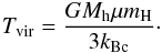 (B.6)Here, Rvir denotes the virial radius of the halo and μ is the mean molecular weight. In this way, we include the velocity distribution of emitters that are gravitationally bound. Photons are emitted from halos with mass ≥5 × 10⁹ M⊙. Since the range of masses and thus intrinsic luminosities is about 3 orders of magnitude, we follow ZCTM10 in applying a weighting procedure for the individual photons to reduce the total number of photons to compute. Each halo emits at least nmin = 1000 photons independently of its mass. In total, we run the RT for about 40 000/49 000/51 000 halos at redshift 4/3/2. To conserve the relative intrinsic luminosities, photons are given a mass-dependent weight.
Appendix B.1: Code verification
To verify the correctness of our radiative transfer code, we perform the standard tests from the literature. In Fig. B.1, the redistribution function f(x,x′) is shown, namely the probability for an infalling photon with frequency x to be reemitted with a frequency x′. In this test, only thermal motions of the scattering atom are considered. Overplotted are the analytical solutions by Lee (1974).
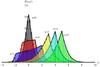 |
Fig. B.1
Comparison of the redistribution function calculated using the analytic solution by Lee (1974) (solid lines) with our code. Shown is the probability that a photon will be reemitted with a frequency x′ when it has the frequency x before the scattering occurs for some values of x. |
| Open with DEXTER | |
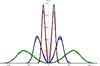 |
Fig. B.2
Comparison between the analytical solution (solid lines) of the spherical test case (see text) and the results obtained by LyS. Shown is the probability distribution of the escaping photons as a function of the dimensionless frequency x. The innermost peaks correspond to an optical depth of 105, the outermost to 107. The third case is for an optical depth of 106. |
| Open with DEXTER | |
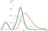 |
Fig. B.3
Dimensionless frequency distribution of photons escaping from an isothermal (2 × 10⁴ K) homogeneous sphere with column density of 2 × 10²⁰NH from the center to the surface. A Hubble-like velocity prescription given by Eq. (B.7) is assigned. The different lines correspond to different maximum collapse velocities: 20 km s-1 (line), 200 km s-1 (dashed), 2000 km s-1 (dotted). |
| Open with DEXTER | |
The standard test for Lyα-codes, the so-called static sphere test, is shown in Fig. B.2 for various optical depths (τ0 = 105/106/107). In this test, photons are launched in the center an isothermal sphere of constant density. Overplotted is the analytic solution from Dijkstra et al. (2006). For these tests, the acceleration scheme was turned off. The static sphere test was also done with the activated acceleration scheme. It still resembles the analytical solution quite well.
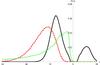 |
Fig. B.4
Same as Fig. B.3, but for an expanding sphere. The different lines correspond to the maximum expansion velocities: 20 km s-1 (line), 200 km s-1 (dashed), 2000 km s-1 (dotted). |
| Open with DEXTER | |
For Figs. B.3 and B.4, the static sphere problem was modified with a Hubble-like bulk velocity field. The gas was assigned a velocity 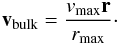 (B.7)Where vmax is a certain constant maximum velocity vmax, r the distance vector from the center of the sphere and rmax the distance from the center where | v | = vmax. Since there is no analytic solution for this test case available, we can only compare the results from other codes. The results from LyS are in good agreement with the plots in Faucher-Giguere et al. (2010) and Dijkstra et al. (2006).
© ESO, 2013
Current usage metrics show cumulative count of Article Views (full-text article views including HTML views, PDF and ePub downloads, according to the available data) and Abstracts Views on Vision4Press platform.
Data correspond to usage on the plateform after 2015. The current usage metrics is available 48-96 hours after online publication and is updated daily on week days.
Initial download of the metrics may take a while.