| Issue |
A&A
Volume 555, July 2013
|
|
|---|---|---|
| Article Number | A27 | |
| Number of page(s) | 9 | |
| Section | The Sun | |
| DOI | https://doi.org/10.1051/0004-6361/201220195 | |
| Published online | 24 June 2013 | |
Online material
Appendix A: Asymptotic solution for large time
In this appendix we study the asymptotic behaviour of the solution to Eq. (29)
for ωt ~ ϵ-1. We introduce the Laplace
transform  (A.1)Applying
the Laplace transform to Eq. (29) and
using the theorem about the Laplace transform of convolution, we obtain
(A.1)Applying
the Laplace transform to Eq. (29) and
using the theorem about the Laplace transform of convolution, we obtain  (A.2)Using
the standard table of Laplace transforms, we find
(A.2)Using
the standard table of Laplace transforms, we find  (A.3)We
do not give the expression
for ℒ [F(t)] (s) because it is
not used in what follows. The solution to Eq. (29) with the initial condition (17) is given by
(A.3)We
do not give the expression
for ℒ [F(t)] (s) because it is
not used in what follows. The solution to Eq. (29) with the initial condition (17) is given by  (A.4)where ς
is any positive constant. When calculating the inverse Laplace transform, we have made
the substitution s = ωs′
and then dropped the prime.
(A.4)where ς
is any positive constant. When calculating the inverse Laplace transform, we have made
the substitution s = ωs′
and then dropped the prime.
Now we use Eq. (A.4) to obtain the
asymptotic expression for η(t) valid
for ωt ~ ϵ-1. The ratio of the second
term in the numerator of the integrand in Eq. (A.4) to the first one is of the order of ϵ. Hence, we can
neglect the second term in the numerator and use the approximate expression
 (A.5)to
calculate the asymptotic behaviour of η(t) at large
time. The integrand in this expression has four logarithmic branch points
at s = ±s+ and
s = ±s−, where
(A.5)to
calculate the asymptotic behaviour of η(t) at large
time. The integrand in this expression has four logarithmic branch points
at s = ±s+ and
s = ±s−, where  (A.6)To
obtain a single-valued branch of the integrand, we make the cuts of the
complex s-plane along the
intervals [−s−, −s+]
and [s+, s−] .
The multivaluedness of the integrand is related to the presence of logarithm in
Eq. (A.3). We define the principal
sheet of the Riemann surface of the integrand by the condition that the imaginary part
of this logarithm is between −πi and πi. In what
follows we use the notation “ln” for this value of logarithm. All other values differ
from this value by 2πni, where n is an integer number.
(A.6)To
obtain a single-valued branch of the integrand, we make the cuts of the
complex s-plane along the
intervals [−s−, −s+]
and [s+, s−] .
The multivaluedness of the integrand is related to the presence of logarithm in
Eq. (A.3). We define the principal
sheet of the Riemann surface of the integrand by the condition that the imaginary part
of this logarithm is between −πi and πi. In what
follows we use the notation “ln” for this value of logarithm. All other values differ
from this value by 2πni, where n is an integer number.
The function  (A.7)maps
the complex s-plane with
cuts [−s−, −s+]
and [s+, s−]
on the
strip −π < ℑ(w) < π
in the complex w-plane, where ℑ indicates the imaginary part of a
quantity. We find the zeros of the denominator of the integrand in Eq. (A.5), which are determined by the equation
(A.7)maps
the complex s-plane with
cuts [−s−, −s+]
and [s+, s−]
on the
strip −π < ℑ(w) < π
in the complex w-plane, where ℑ indicates the imaginary part of a
quantity. We find the zeros of the denominator of the integrand in Eq. (A.5), which are determined by the equation
 (A.8)Let s∗
be a root of this equation. If it is not close to ±s±
then it follows that
(A.8)Let s∗
be a root of this equation. If it is not close to ±s±
then it follows that  . This implies that
either
. This implies that
either  or
or  .
In the first case we immediately see that the left-hand side of Eq. (A.8) is of the order
of ϵ2, so that the only possible solution of this kind
is s∗ = 0.
Since ℒ [G(t)] (0) = κ, it is
straightforward to see that the denominator of the integrand in Eq. (A.5) does not equal zero
when s = 0. Hence, s∗ = 0 is a spurious
root.
.
In the first case we immediately see that the left-hand side of Eq. (A.8) is of the order
of ϵ2, so that the only possible solution of this kind
is s∗ = 0.
Since ℒ [G(t)] (0) = κ, it is
straightforward to see that the denominator of the integrand in Eq. (A.5) does not equal zero
when s = 0. Hence, s∗ = 0 is a spurious
root.
Considering the second possibility, namely, ,
we look for the root to Eq. (A.8) in the
form s∗ = ±1 + ϵδ. By substituting
this expression in Eq. (A.8) we obtain
 (A.9)The
imaginary part of the left-hand side of this equation is close to −πi
when ℑ(±δ) < 0 and to πi
when ℑ(±δ) > 0. This implies that the
imaginary parts of the left- and right-hand side of Eq. (A.9) have different signs, so that this equation cannot have a
solution with ℑ(δ) ≠ 0. It also cannot have a real solution because in
that case the imaginary part of the right-hand side is zero, while the imaginary part of
the left-hand side is non-zero.
(A.9)The
imaginary part of the left-hand side of this equation is close to −πi
when ℑ(±δ) < 0 and to πi
when ℑ(±δ) > 0. This implies that the
imaginary parts of the left- and right-hand side of Eq. (A.9) have different signs, so that this equation cannot have a
solution with ℑ(δ) ≠ 0. It also cannot have a real solution because in
that case the imaginary part of the right-hand side is zero, while the imaginary part of
the left-hand side is non-zero.
Hence, Eq. (A.8) can only have
solutions close to ±s±. We look for the solution in the
form s∗ = ±s± + δ,
where δ ≪ 1. Substituting this expression in Eq. (A.8) we obtain four
roots,  and
and  ,
where
,
where  (A.10)Hence,
there are four poles on the real axis, at
and .
(A.10)Hence,
there are four poles on the real axis, at
and .
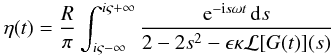
The integration contour in Eq. (A.5) is a straight line parallel to the real axis. Its equation in ℑ(s) = ς > 0. Since the integrand in Eq. (A.5) is an analytical function in the upper part of the complex s-plane, we can deform the integration contour arbitrarily without changing the value of the integral. The only conditions that have to be satisfied are that the new contour is completely in the union of the upper part of the complex s-plane and the real axis and that the part of the new contour that is on the real axis does not contain singularities of the integrand. It is convenient to use the new integration contour shown in Fig. A.1. This contour consists
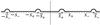 |
Fig. A.1
Integration contour used to obtain Eq. (A.11) is shown by the thick solid line. The dashed lines show the cuts. |
| Open with DEXTER | |
of five intervals of the real axis,  ,
,
 ,
,
 ,
,
 ,
and
,
and  ,
and four half-circles of radius ε centred
at
,
and four half-circles of radius ε centred
at  and
and  .
Taking ε → +0 we obtain
.
Taking ε → +0 we obtain 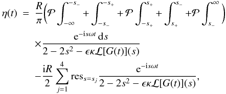 (A.11)where
  ,
,  ,
,  indicates the principal Cauchy part of an integral, and in the integrals along the
intervals [−s−, −s+]
and [s+, s−]
the integrand is calculated at the upper edges of the cuts.
indicates the principal Cauchy part of an integral, and in the integrals along the
intervals [−s−, −s+]
and [s+, s−]
the integrand is calculated at the upper edges of the cuts.
First of all, we note that 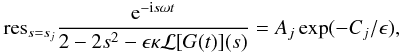 (A.12)where j = 1,2,3,4, Aj
and Cj are constants of the order of
unity, and Cj > 0.
This implies that the contribution of the last term in Eq. (A.11) is exponentially small and can be
neglected. Using the integration by parts we obtain
(A.12)where j = 1,2,3,4, Aj
and Cj are constants of the order of
unity, and Cj > 0.
This implies that the contribution of the last term in Eq. (A.11) is exponentially small and can be
neglected. Using the integration by parts we obtain 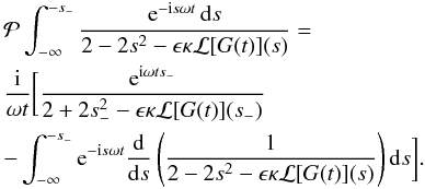 (A.13)We
see that the contribution of the integral along the
interval (−∞, −s−] is of the order
of 1/ωt. Similarly we can show that the
contribution of the integrals along the
intervals [−s+, s+]
and [s−, ∞) are also of the order
of 1/ωt. Hence, we obtain
(A.13)We
see that the contribution of the integral along the
interval (−∞, −s−] is of the order
of 1/ωt. Similarly we can show that the
contribution of the integrals along the
intervals [−s+, s+]
and [s−, ∞) are also of the order
of 1/ωt. Hence, we obtain  (A.14)To
evaluate the asymptotic behaviour of the integrals in this expression, we need to make
the analytic continuation of the function w(s) on its
Riemann surface. This Riemann surface consists of an infinite set of complex planes with
cuts [−s−, −s+]
and [s+, s−]
properly attached to each other at the cuts. In what follows we use only two
non-principal sheets of the Riemann surface attached to the principal sheet at the upper
edges of the cuts. To define w(s) on the non-principal
sheet of the Riemann surface attached to the principal sheet at the upper edge of the
right cut, we consider a point s near this cut on the principal sheet.
We
write s = sr + isi,
where s+ < sr < s−
and |si| ≪ sr. Then
(A.14)To
evaluate the asymptotic behaviour of the integrals in this expression, we need to make
the analytic continuation of the function w(s) on its
Riemann surface. This Riemann surface consists of an infinite set of complex planes with
cuts [−s−, −s+]
and [s+, s−]
properly attached to each other at the cuts. In what follows we use only two
non-principal sheets of the Riemann surface attached to the principal sheet at the upper
edges of the cuts. To define w(s) on the non-principal
sheet of the Riemann surface attached to the principal sheet at the upper edge of the
right cut, we consider a point s near this cut on the principal sheet.
We
write s = sr + isi,
where s+ < sr < s−
and |si| ≪ sr. Then
 (A.15)and
we obtain
(A.15)and
we obtain  (A.16)We
assume that a point s on the principal Riemann sheet moves in such a
way that it crosses the right cut from the upper to the lower part of the complex plane,
i.e. ℑ(s) changes the sign from positive to negative. Then Eq. (A.16) implies that ℑ(w)
jumps by −2πi during this crossing. This means that to have the
continuous change of w(s) when s
moves from the upper part of the principal Riemann sheet to the lower part of the
non-principal Riemann sheet we have to define w(s) on
this non-principal sheet as
(A.16)We
assume that a point s on the principal Riemann sheet moves in such a
way that it crosses the right cut from the upper to the lower part of the complex plane,
i.e. ℑ(s) changes the sign from positive to negative. Then Eq. (A.16) implies that ℑ(w)
jumps by −2πi during this crossing. This means that to have the
continuous change of w(s) when s
moves from the upper part of the principal Riemann sheet to the lower part of the
non-principal Riemann sheet we have to define w(s) on
this non-principal sheet as  (A.17)In
a similar way we find that the analytic continuation
of w(s) on the non-principal Riemann sheet attached
to the principal sheet at the upper edge at the left cut is defined by
(A.17)In
a similar way we find that the analytic continuation
of w(s) on the non-principal Riemann sheet attached
to the principal sheet at the upper edge at the left cut is defined by  (A.18)To
calculate the integral along the
interval [s+, s−]
in Eq. (A.14), we use the contour shown
in Fig. A.2. It consists of the
interval [s+, s−]
at the upper edge of the right cut on the principal Riemann sheet, two vertical lines
from s+
to s+ − ib and
from s−
to s− − ib on the non-principal Riemann
sheet, and the horizontal line connecting the
points s+ − ib
and s− − ib, once again on the
non-principal Riemann sheet. Here b > 0. To
calculate the integral along this contour we need to find the poles of the integrand
inside this contour. These poles coincide with the zeros
(A.18)To
calculate the integral along the
interval [s+, s−]
in Eq. (A.14), we use the contour shown
in Fig. A.2. It consists of the
interval [s+, s−]
at the upper edge of the right cut on the principal Riemann sheet, two vertical lines
from s+
to s+ − ib and
from s−
to s− − ib on the non-principal Riemann
sheet, and the horizontal line connecting the
points s+ − ib
and s− − ib, once again on the
non-principal Riemann sheet. Here b > 0. To
calculate the integral along this contour we need to find the poles of the integrand
inside this contour. These poles coincide with the zeros
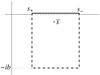 |
Fig. A.2
Integration contour used to calculate the integral along the interval [s+, s−] in Eq. (A.14). The solid line indicates the part of the contour that coincides with the upper edge of the right cut on the principal Riemann sheet. The dashed-dotted line indicates the parts of the contour on the non-principal Riemann sheet. The dashed line shows the cut. |
| Open with DEXTER | |
of Eq. (A.8). Since the area enclosed by the contour is on the non-principal Riemann sheet, we look for zeros of Eq. (A.8) on this sheet.
Although w(s) is now not given by Eq. (A.7) but by Eq. (A.17), the roots of Eq. (A.8) are still close to either 0 or 1 or to
one of the numbers ±s±. Obviously, the root close to 0
cannot be inside the contour. Simple analysis shows that there are roots close
to ±s− and ±s+, but
their real parts are equal to
and ,
respectively, so these roots are also not inside the contour. Finally, the root close
to 1 is given by 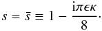 (A.19)This
root is inside the contour. Hence,
(A.19)This
root is inside the contour. Hence,
 (A.20)We
estimate the integrals along the parts of the closed contour that are on the
non-principal Riemann sheet. Using the integration by parts we have
(A.20)We
estimate the integrals along the parts of the closed contour that are on the
non-principal Riemann sheet. Using the integration by parts we have  (A.21)where
the limit is taken as b → ∞. In the same way we prove that the integral
along the vertical line connecting the
points s+ − ib
and s+ is of the order
of 1/ωt. Finally, the integral along the
horizontal line connecting the
points s− − ib
and s+ − ib tends to zero
as b → ∞. As a result we have
(A.21)where
the limit is taken as b → ∞. In the same way we prove that the integral
along the vertical line connecting the
points s+ − ib
and s+ is of the order
of 1/ωt. Finally, the integral along the
horizontal line connecting the
points s− − ib
and s+ − ib tends to zero
as b → ∞. As a result we have  (A.22)}where
 is a
complex constant. In a similar way we can obtain a similar expression for the integral
along the
interval [−s−, −s+] .
is a
complex constant. In a similar way we can obtain a similar expression for the integral
along the
interval [−s−, −s+] .
It is worth explaining why we cannot prove in the same way that the integral along the interval [s+, s−] is of the order of 1/ωt.
The reason is that there is a pole at  ,
which is close to the
interval [s+, s−] .
After the integration by parts we obtain 1/ωt times
an integral. The integrand in this integral is very big, in the vicinity
of s = 1, so the whole product is not of the order
of 1/ωt.
,
which is close to the
interval [s+, s−] .
After the integration by parts we obtain 1/ωt times
an integral. The integrand in this integral is very big, in the vicinity
of s = 1, so the whole product is not of the order
of 1/ωt.
Summarising the analysis of this section, we arrive at the asymptotic expression
 (A.23)where C
is a complex constant and c.c. denotes complex conjugate.
(A.23)where C
is a complex constant and c.c. denotes complex conjugate.
© ESO, 2013
Current usage metrics show cumulative count of Article Views (full-text article views including HTML views, PDF and ePub downloads, according to the available data) and Abstracts Views on Vision4Press platform.
Data correspond to usage on the plateform after 2015. The current usage metrics is available 48-96 hours after online publication and is updated daily on week days.
Initial download of the metrics may take a while.