| Issue |
A&A
Volume 554, June 2013
|
|
|---|---|---|
| Article Number | A100 | |
| Number of page(s) | 32 | |
| Section | Interstellar and circumstellar matter | |
| DOI | https://doi.org/10.1051/0004-6361/201220959 | |
| Published online | 11 June 2013 | |
Online material
Appendix A: Detected lines per species for all sources
The line assignment and detection is based on Gaussian fitting with the following criteria: (i) the fitted line position has to be within ±1 MHz of the catalog frequency; (ii) the FWHM is consistent with the those given in Table 1; and (iii) the peak intensity has at least a S/N = 3. The errors on the integrated intensities are computed as follows.
The integrated main beam temperatures,  , were obtained by Gaussian fits to the lines (Eq. (A.1)).
 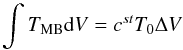 (A.1)with
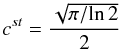 where T0 is the peak intensity and ΔV is the FWHM of the line. The error,
  , is calculated from Eq. (A.2).
 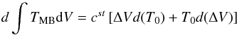 (A.2)with
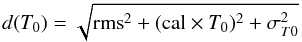
 where rms is the root mean square amplitude of the noise in the spectral bin δv, cal is the calibration uncertainty of the telescope, and σ’s are the statistical errors on T0 and ΔV from the Gaussian fits.
The errors on the integrated intensities derived from Eq. (A.2) include all statistical errors from the Gaussian fit.  (A.3)For undetected transitions the upper limits were determined as 3σ limits (Eq. (A.4)) using:
  (A.4)where 1.2 is the coefficient related to the calibration uncertainty of 20%.
CLASS was used to determine the Gaussian fits and the uncertainties in the individual parameters. The formal errors on the integrated intensities derived from Eq. (A.3) in some cases yield a S/N < 2.5. This is caused by: (i) a conservative estimate of the statistical error on the FWHM parameter in the Gaussian fitter of CLASS; (ii) all statistical errors are included into our error calculation. Considering the higher S/N on the peak intensity, a more traditional error estimate without the statistical errors from the Gaussian fit (Eq. (A.3)) would result in a S/N > 3 for the integrated intensity as well. All weak line fits were confirmed by visual inspection.
Observed line fluxes  (K km s-1) for H2CO and its isotopic species.
Observed line fluxes (K km s-1) for CH3OH and its isotopic species.
Observed line fluxes (K km s-1) for C2H5OH.
Observed line fluxes (K km s-1) for HNCO and its isotopic species.
Observed line fluxes (K km s-1) for NH2CHO.
Observed line fluxes (K km s-1) for CH3CN and its isotopic species.
Observed line fluxes (K km s-1) for C2H5CN.
Observed line fluxes (K km s-1) for HCOOCH3.
Observed line fluxes (K km s-1) for HCOOCH3 continued.
Observed line fluxes (K km s-1) for CH3OCH3.
Observed line fluxes (K km s-1) for CH2CO.
Observed line fluxes (K km s-1) for CH3CHO.
Observed line fluxes (K km s-1) for HCOOH and its isotopic species.
Observed line fluxes (K km s-1) for CH3CCH.
Appendix B: Rotation diagrams
RTD diagrams for H2CO, CH3OH, C2H5OH, HNCO, NH2CHO, CH3CN, C2H5CN, HCOOCH3, CH3OCH3, CH2CO and CH3CCH. Lines from different frequency bands are corrected for differential beam dilution assuming a RT = 100 K source size for the warm species and 14″ source size for the cold species, as indicated in the plots. Optically thin, unblended lines with S/N ≳ 2 are marked with filled circles. Lines with high S/N (≲2) are marked with diamonds, those included in the fit with filled diamonds. Optically thick lines and blended lines are marked with open squares and triangles, respectively. Upper limits are marked with arrows. Upper limits used to constrain the fit are marked with filled stars. The error bars are calculated using Eq. (A.2).
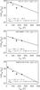 |
Fig. B.1
RTD fits for H2CO. All lines included into the fit belong to para-H2CO. |
| Open with DEXTER | |
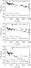 |
Fig. B.2
RTD fits for CH3OH. Lines with Eup < 100 K are considered contaminated with the cold CH3OH. Lines with S/N ≳ 1 are included in the fit. |
| Open with DEXTER | |
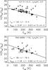 |
Fig. B.3
RTD fits for C2H5OH. No C2H5OH was detected in IRAS 20126+4104. For IRAS 18089 lines with S/N ≳ 1 have been used. |
| Open with DEXTER | |
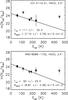 |
Fig. B.4
RTD fits for HNCO. No HNCO was detected in IRAS 20126+4104. |
| Open with DEXTER | |
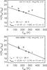 |
Fig. B.5
RTD fits for NH2CHO. No NH2CHO was detected in IRAS 20126+4104. |
| Open with DEXTER | |
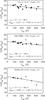 |
Fig. B.6
RTD fits for CH3CN. |
| Open with DEXTER | |
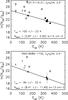 |
Fig. B.7
RTD fits for C2H5CN. No C2H5CN was detected in IRAS 20126+4104. For IRAS 18089 lines with S/N ≲ 2 have been included in the fit. |
| Open with DEXTER | |
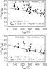 |
Fig. B.8
RTD fits for HCOOCH3. No HCOOCH3 was detected in IRAS 20126+4104. |
| Open with DEXTER | |
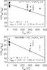 |
Fig. B.9
RTD fits for CH3OCH3. No CH3OCH3 was detected in IRAS 20126+4104. |
| Open with DEXTER | |
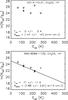 |
Fig. B.10
RTD fits for CH2CO. No CH2CO was detected in IRAS 20126+4104. |
| Open with DEXTER | |
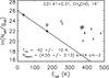 |
Fig. B.11
RTD fits for CH3CHO. |
| Open with DEXTER | |
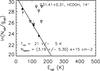 |
Fig. B.12
RTD fits for HCOOH. |
| Open with DEXTER | |
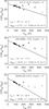 |
Fig. B.13
RTD fits for CH3CCH. |
| Open with DEXTER | |
Appendix C: Weeds model parameters
Weeds model parameters for IRAS 20126+4104.
Weeds model parameters for IRAS 18089-1732.
Weeds model parameters for G31.41+0.31.
Appendix D: Additional detections
Several lines of other species were found in the observed frequency ranges, particularly in the line-rich G31.41+0.31. Table D.1 lists additional detections with column densities obtained from the Weeds analysis with the best Tex when this could be derived. Several transitions of acetone, CH3COCH3, are detected. In G31, the best agreement is obtained at 100 K, whereas for IRAS 18089, this is Tex = 300 K. No CH3COCH3 was detected in IRAS 20126, and the tabulated value is an upper limit at 300 K. Figure D.1 shows the strongest acetone lines in G31 together with the Weeds model.
 |
Fig. D.1
Beam-averaged spectra of CH3COCH3 (231/2,22,1–221/2,21,1), (231/2,22,0–221/2,21,1), (287/8,21,0–278/7,20,0) and (287/8,21,0–278/7,20,1) towards G31.41+0.31 hot core. Dashed lines indicate Gaussian fits to the lines and red solid line show the Weeds model on the CH3COCH3 lines at 100 K. |
| Open with DEXTER | |
Glycoaldehyde, HCOCH2OH, has previously been detected in G31 (Beltrán et al. 2009), has several lines in the covered ranges. All lines are however blended with other transitions, and only upper limit could therefore be derived reliably. The tabulated column density is for a temperature of 300 K, constrained by non-detection of lines with low Eup.
Two transitions of HC3N are detected at 218.325 GHz (Eup131.0 K) (J = 24 → 23) and 354.697 GHz (Eup340.5 K) (J = 39 → 38). The Weeds model on the two lines, well separated in Eup, gives a beam averaged column density of 7 × 1013 cm-2 and a temperature of 150 K for G31. The HC3N emission cannot be matched with emission contained within a 2.0″ volume as the low-Euptransition becomes optically thick. For IRAS 20126, the tabulated column density is at 100 K, constrained by the two transitions. Only the high Eup transition was covered for IRAS 18089 giving a column density of 3 × 1013 cm-2 at 150 K and 6 × 1013 cm-2 at 100 K.
Several CH3NH2 transitions are observed with a Tex of 150 K. Blends with other species make the rotation temperature and column density inaccurate, however. Several unidentified lines coincide with NH2CH2CH2OH, but only upper limits of 1.0× 1016 cm-2 at 100-300 K could be derived reliably using Weeds.
Several weak lines of NH2CN are detected, with a Tex of 50 K derived from the Weeds model, but line blends make the rotation temperature and column density inaccurate. For CN, SO, 34SO, O13CS, OC34S, SO2, 33SO2, C34S, and CP not enough lines were observed to derive Tex values, and tabulated column densities are assuming a temperature of 50 K.
One line of HCN, J = 4–3, was observed. HCN emission in G31 is composed of a broad (12 km s-1) and a narrow (6 km s-1) component (redshifted by 2.5 km s-1) causing self-absorption. For IRAS 18089, the broad component has a width of 7 km s-1 and narrow 4 km s-1 (redshifted by 1 km s-1). For IRAS 20126 the HCN emission has a very broad 20 km s-1 component blueshifted by 2 km s-1 and a narrow (5 km s-1) component redshifted by 1 km s-1. The tabulated column densities are those derived from the H13CN column density.
Additional detections. Column densities given are source averaged for species with Tex> 100 K and beam averaged for species with Tex< 100 K (except for HCCCN, the emission of which is warm and arises from extended volume). The tabulated values are those obtained from Weeds analysis with the best Tex.
© ESO, 2013
Current usage metrics show cumulative count of Article Views (full-text article views including HTML views, PDF and ePub downloads, according to the available data) and Abstracts Views on Vision4Press platform.
Data correspond to usage on the plateform after 2015. The current usage metrics is available 48-96 hours after online publication and is updated daily on week days.
Initial download of the metrics may take a while.