| Issue |
A&A
Volume 553, May 2013
|
|
|---|---|---|
| Article Number | A38 | |
| Number of page(s) | 14 | |
| Section | The Sun | |
| DOI | https://doi.org/10.1051/0004-6361/201220982 | |
| Published online | 29 April 2013 | |
Online material
Appendix A: Details of the numerical implementation
In the applications presented in this paper we have considered uniform Cartesian grids
of resolution Δ in all directions, discretizing a rectangular volume
 (see Sect. 4 for the actual values of Δ and
in each case). We compute derivatives using the standard second-order,
central-difference operator, and we employ the relevant one-sided (i.e., forward or
backward), second-order differences at the boundaries of
.
The only exception is the computation of the divergence of
Btest, since all test fields are known in a volume that is
larger than the selected
(on lateral and top boundaries). In this case, ∇·Btest is
computed using the central differences also at the location of the lateral and top
boundaries of .
(see Sect. 4 for the actual values of Δ and
in each case). We compute derivatives using the standard second-order,
central-difference operator, and we employ the relevant one-sided (i.e., forward or
backward), second-order differences at the boundaries of
.
The only exception is the computation of the divergence of
Btest, since all test fields are known in a volume that is
larger than the selected
(on lateral and top boundaries). In this case, ∇·Btest is
computed using the central differences also at the location of the lateral and top
boundaries of .
In the computation of volume integrals, the cell volume Δ3 is assigned to
each internal node of the grid, whereas the cell volume is reduce to half, one fourth,
and one eighth for nodes on the lateral surfaces, edges, and corners of
,
respectively. Similarly, in the computation of surface integrals, the cell surface
Δ2 is assigned to each node inside each side of
,
whereas the cell surface is reduced to half and one fourth on edges and corners of each
side, respectively. Despite the accurate computation of integrals, the divergence
theorem, Eq. (4), is not insured to hold
numerically, a property that requires special techniques, like finite-volume
discretizations, to be fulfilled.
Appendix B: Divergence cleaner
To construct a numerically solenoidal field [Bs] from a field
[B] let us define  (B.1)where A
is the vector potential computed from B in the volume
(B.1)where A
is the vector potential computed from B in the volume
 .
The vector potential A can be derived as in Valori et al. (2012) using the gauge ẑ·A = 0,
yielding the expression
.
The vector potential A can be derived as in Valori et al. (2012) using the gauge ẑ·A = 0,
yielding the expression 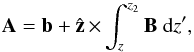 (B.2)where
b ≡ (Ax(x,y,z = z2),Ay(x,y,z = z2),0)
is any solution of
(B.2)where
b ≡ (Ax(x,y,z = z2),Ay(x,y,z = z2),0)
is any solution of  (B.3)A direct substitution
of Eq. (B.2) into Eq. (B.1) shows that
(B.3)A direct substitution
of Eq. (B.2) into Eq. (B.1) shows that 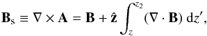 (B.4)with the property that
∇·Bs = 0. In other words, Eq. (B.4) naturally separates B into a solenoidal part
Bs and a nonsolenoidal one, thus defining a
divergence cleaner for B. The z-component of
B is changed throughout the volume except on the top boundary, whereas
the x- and y-components are unchanged. The amplitude
of the modification to B at a given height z is given by
the cumulative effect of “magnetic charges” above that altitude.
(B.4)with the property that
∇·Bs = 0. In other words, Eq. (B.4) naturally separates B into a solenoidal part
Bs and a nonsolenoidal one, thus defining a
divergence cleaner for B. The z-component of
B is changed throughout the volume except on the top boundary, whereas
the x- and y-components are unchanged. The amplitude
of the modification to B at a given height z is given by
the cumulative effect of “magnetic charges” above that altitude.
Since only the z-component of the field is changed, the divergence
cleaner changes the x- and y-components of the
current, but not the z-component, 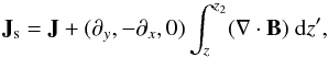 (B.5)
(B.5)
therefore the cleaner changes the injected magnetic flux but not the injected electric current through the bottom layer. On the other hand, since most of the test fields considered in this article have the highest values of divergence close to the bottom boundary, only the lower part of the field is changed significantly by the cleaner.
Computation Bs requires numerical computation of an integral of
the type  , as
in Eq. (B.4) for
f = ∇·B. To achieve numerical accuracy in the solenoidal
property of Bs, G(z) must
satisfy
∂zG(z) = −f(z)
numerically, i.e., must satisfy the numerical formulation of the fundamental theorem of
integral calculus in the employed discretization. For the second-order central
differences that are used in the analysis, this can be obtained by the recurrence
formulae
, as
in Eq. (B.4) for
f = ∇·B. To achieve numerical accuracy in the solenoidal
property of Bs, G(z) must
satisfy
∂zG(z) = −f(z)
numerically, i.e., must satisfy the numerical formulation of the fundamental theorem of
integral calculus in the employed discretization. For the second-order central
differences that are used in the analysis, this can be obtained by the recurrence
formulae 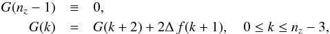 (B.6)where
G(z) = G(z1 + kΔ) ≡ G(k)
with
k = 0,1,2,··· ,(nz − 1),
and Δ is the uniform spatial resolution in z.
(B.6)where
G(z) = G(z1 + kΔ) ≡ G(k)
with
k = 0,1,2,··· ,(nz − 1),
and Δ is the uniform spatial resolution in z.
The constraint
∂zG(z) = −f(z)
in the second-order, central-difference discretization does not fix the value of
G(nz − 2). To do that,
we require that the divergence of Eq. (B.4) also vanishes at the bottom boundary, i.e.,
(∇·Bs)|z = z1 = 0.
Here the second-order divergence operator is computed by using a second-order, forward
derivative in the z-direction, i.e., defining the operator
 , where
 and
and  . By
using the recurrence formula Eq. (B.6),
the condition on the bottom boundary is transformed into the condition for
G(nz − 2), yielding
. By
using the recurrence formula Eq. (B.6),
the condition on the bottom boundary is transformed into the condition for
G(nz − 2), yielding
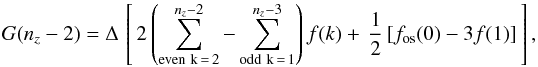 where
fos = ∇os·B. Such a numerical
trick is only possible if the volume is discretized by an even number of points in the
z-direction, therefore the analysis volumes employed in the article
were chosen to satisfy such a requirement.
where
fos = ∇os·B. Such a numerical
trick is only possible if the volume is discretized by an even number of points in the
z-direction, therefore the analysis volumes employed in the article
were chosen to satisfy such a requirement.
Appendix C: Measures of ∇ · B
The total divergence of a field B can be conveniently expressed by a
single number using the average
⟨ |fi| ⟩ over the grid nodes of
the fractional flux 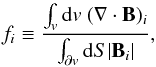 (C.1)through the surface
∂v of a small volume v including the node
i (Wheatland et al. 2000).
Taking a cubic voxel of side equal to Δ as the small volume v centered
on each node, the divergence in the discretized volume
of uniform and homogeneous resolution Δ is then given by
(C.1)through the surface
∂v of a small volume v including the node
i (Wheatland et al. 2000).
Taking a cubic voxel of side equal to Δ as the small volume v centered
on each node, the divergence in the discretized volume
of uniform and homogeneous resolution Δ is then given by 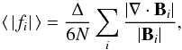 (C.2)where
i runs over all N nodes in
.
This metric depends on the considered volume, so that values are strictly comparable
only if computed on equal volumes.
(C.2)where
i runs over all N nodes in
.
This metric depends on the considered volume, so that values are strictly comparable
only if computed on equal volumes.
© ESO, 2013
Current usage metrics show cumulative count of Article Views (full-text article views including HTML views, PDF and ePub downloads, according to the available data) and Abstracts Views on Vision4Press platform.
Data correspond to usage on the plateform after 2015. The current usage metrics is available 48-96 hours after online publication and is updated daily on week days.
Initial download of the metrics may take a while.