| Issue |
A&A
Volume 540, April 2012
|
|
|---|---|---|
| Article Number | A2 | |
| Number of page(s) | 21 | |
| Section | Interstellar and circumstellar matter | |
| DOI | https://doi.org/10.1051/0004-6361/201117624 | |
| Published online | 13 March 2012 | |
Online material
Appendix A: Tauc analysis of the avaialble data
In Sect. 3 we showed how optical data can be fitted, and the band gap (Tauc gap) determined, using the linear portion of a Tauc plot, i.e. (αE)0.5 vs. E. At higher and lower energies the behaviour deviates from this linear trend but can be extended to lower energies with the addition of an exponential Urbach tail contribution (see Sect. 3.1). At higher energies the data can be fitted, for aesthetic purposes only (see Sect. 3.1), with  (A.1)where the left-hand term is the linear portion and the right hand is an “inversed gaussian tail” fit to the data. Table A.1 lists the adopted values for the parameters EUV and σUV.
We have appled this “Tauc analysis” to the available laboratory-measured and modelled optical data (Smith 1984; Rouleau & Martin 1991; Mennella et al. 1995; Zubko et al. 1996, and DDOP) and have derived the parameters for the Tauc fits, these are given in Table A.2. The derived values for B shown in Table A.2 are in good agreement with those expected for these materials, i.e., ≃ 4 × 10⁴ eV-1 cm-1 for a-C and ≃ 6 × 10⁴ eV-1 cm-1 for a-C:H (Robertson 1986). Additionally, and as Robertson (1986) points out, Eg is a measure of the largest significant aromatic cluster size and B gives the range of cluster sizes. In the accompanying figures (Fig. 5 and Figs. A.1 to A.4) we show these fits along with the optEC(s) model data. We recall here that we have colour-coded the data (see Table 1) in order to facilitate the comparison between the model and laboratory data.
As can be seen, by comparing these colour-coded data, the optEC(s) model, qualitatively at least, follows all of the major trends in these data over the entire visible-UV wavelengths region.
However, certain laboratory and modelled data appear to deviate from the general trends when plotted in this way. We do not here wish to enter into any speculations as to why this might be the case, other than by referring to the comments about possible electrical conductivity effects mentioned in the following Appendix.
The Tauc analysis-derived parameters for the optical data in the given references.
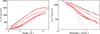 |
Fig. A.1
The laboratory data from (Mennella et al. 1995, (coloured curves with small data points)) plotted as (αE)0.5 vs. energy, Tauc plot (upper), and also versus wavelength (lower). The red lines show the modelled fits to the data using Eqs. (8) and (9), with the addition of an “inverse Gaussian tail” at high energies. The red squares delineate the portion used to determine B and the extrapolation to Eg (dashed red lines). The black squares indicate the transition energies to the Urbach tail, E1. The lines without data points are the optEC(s) model data. |
| Open with DEXTER | |
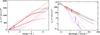 |
Fig. A.2
As per Figs. 5 and A.1 but for the Rouleau & Martin (1991) data. |
| Open with DEXTER | |
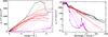 |
Fig. A.3
As per Fig. A.1 but for the Jena DDOP amorphous carbon data. Also shown for comparison are the data for graphite using the usual |
| Open with DEXTER | |

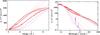 |
Fig. A.4
As per Fig. A.1 but for the Zubko et al. (1996) data. |
| Open with DEXTER | |
Appendix B: The derived optical constants compared with the available data
In Figs. B.1 to B.5 we present the real and imaginary parts of the complex refractive index for the available laboratory and modelled data (Duley 1984; Smith 1984; Rouleau & Martin 1991; Mennella et al. 1995; Zubko et al. 1996, and DDOP) compared to the optEC(s) model-derived values.
 |
Fig. B.1
The imaginary (upper) and real (lower) parts of the refractive index for the Smith (1984) data (lines with data points) compared to the optEC(s) model data (lines without data points). The solid black lines with data points show the Duley (1984) a-C k (upper) and n data (lower); for comparison purposes only, the dashed line shows the n data shifted down by 0.75. |
| Open with DEXTER | |
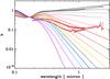 |
Fig. B.2
Same as Fig. B.1 but for the Mennella et al. (1995) data. |
| Open with DEXTER | |
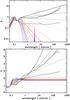 |
Fig. B.3
Same as Fig. B.1 but for the Rouleau & Martin (1991) data. |
| Open with DEXTER | |
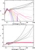 |
Fig. B.4
Same as Fig. B.1 but for the Jena DDOP amorphous carbon data. |
| Open with DEXTER | |
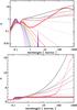 |
Fig. B.5
Same as Fig. B.1 but for the Zubko et al. (1996) data. |
| Open with DEXTER | |
Clearly the optEC(s) model reproduces all of the observed trends in the laboratory and the other modelled data extremely well, however, the data do fall “short” in explaining all of the long wavelength optical property behaviour. For example, looking at the DDOP k data presented in Fig. B.4, in particular in the 100 μm region, it is clear that there appear to be other bands that contribute to the long wavelength behaviour in these samples. However, it should be pointed out that the presence of structure at ≈3,10 and 100 μm, and perhaps some other underlying broad structures, is rather reminiscent of water ice bands at ≈3,6,12,44 and 100 μm. Thus, it is possible that some of the features present in these data could be due to adsorbed water in the samples but this possibility needs to be eliminated. We have therefore not tried to fit the ≈100 μm band, or indeed any others that might contribute at long wavelengths (in these and the other data), and advise that until such time as the exact origin of these bands is understood and quantified it is rather premature to do so.
We also note that there is present, to a greater or lesser extent, an “upward” curvature in some of the laboratory k data. This kind of behaviour, especially evident in the Mennella et al. (1995) and Rouleau & Martin (1991) data (the latter being derived from an earlier version of the data in Mennella et al. 1995), is reminiscent of an electrical conductivity contribution, such as seen in the graphite k data, and we therefore suspect that inter-particle electrical conduction may be playing a role here. Conduction between particles is notoriously difficult to eliminate in these demanding experimental measurements. Thus, it may not be too surprising to see residual electrical conductivity effects in these data arising from un-wanted particle clustering in the laboratory samples.
Zubko et al. (1996) took careful account of the clustering effects in their data analysis and modelling and this is evident in their AC1 and ACAR data, which show clear linear tendencies from FIR to mm wavelengths with no indication of an “upturn” in the k data. Hence, it appears that particle clustering (and the associated conductivity effect) could indeed be the origin of the FIR-mm “upturn”. Rouleau & Martin (1991) also made allowance for particle clustering effects but arrived at rather different results.
In the DDOP data this “upward” curvature is apparent in the n data, which perhaps indicates that in these data, at least, the curvature in the k data is due to the presence of the long wavelength bands. That the long wavelength wings of, as-yet uncharacterised, FIR bands can contribute to the behaviour in the FIR-cm region will have major implications for the observed dust emissivity, as it would lead to a flattening of the carbonaceous dust emissivity at these wavelengths. Thus, and until such time as these bands are well characterised by laboratory measurements, some caution should be exercised in the use of these optEC(s) model data at mm wavelengths and beyond.
© ESO, 2012
Current usage metrics show cumulative count of Article Views (full-text article views including HTML views, PDF and ePub downloads, according to the available data) and Abstracts Views on Vision4Press platform.
Data correspond to usage on the plateform after 2015. The current usage metrics is available 48-96 hours after online publication and is updated daily on week days.
Initial download of the metrics may take a while.