| Issue |
A&A
Volume 537, January 2012
|
|
|---|---|---|
| Article Number | L8 | |
| Number of page(s) | 7 | |
| Section | Letters | |
| DOI | https://doi.org/10.1051/0004-6361/201118358 | |
| Published online | 17 January 2012 | |
Online material
Appendix A: Details of the spectral fitting
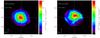 |
Fig. A.1
Flux maps of the broad (B, left) and narrow (A, right) components of [OIII]. |
| Open with DEXTER | |
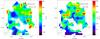 |
Fig. A.2
Velocity field (left) and velocity dispersion (right) of the narrow component (A*) of Hα. |
| Open with DEXTER | |
Results of the spectral fit for the individual components.
The initial spectral fit is performed on a spectrum extracted from a central aperture of ten pixels (i.e. 0.5 arcsec) in the H band and 20 pixels (i.e. 1.0 arcsec) in the K band, which guarantee high S/N.
The emission lines are fitted with multiple Gaussians and, in the case of the broad lines, by also using power-law profiles, as in Nagao et al. (2006). The continuum is fitted with a single power law, which represents the emission of the QSO accretion disk (plus possibly some minor contribution from the host galaxy stellar continuum). Starting from this initial fit in the central region, we fitted the spectra individually at all spatial pixels by leaving most of the parameters free, except for the velocity, dispersion, and relative intensity of the components describing the broad lines (Hα and Hβ). Indeed, since the BLR is unresolved, the shape and shift of the broad line profile (components C+D+E in the case of Hβ) must be constant over the field of view, and there the global intensity variation only reflects the seeing PSF. We tried to also include an Fe II template in the spectral fitting (as in Netzer et al. 2004); however, this is always set to zero by the fitting procedure, confirming the lack of significant FeII emission inferred by the visual inspection of the spectrum. This result contrasts with the measurement of Netzer et al. (2004), who obtain a flux of the Fe II emission that is about 0.37 times the Hβ emission, and we ascribe the discrepancy to the much lower signal-to-noise in the latter spectrum.
Figure 1 shows the various components used to fit the H-band spectrum of the central region and, in the bottom panel, the fit residuals. The region included within the two green lines is affected by strong sky residuals and was not considered in the fit. In this figure we can see that the [OIII] profile can be nicely fitted with two Gaussians, one relatively narrow (A, FWHM ~ 600 km s-1) and a second one (B) blueshifted by about 700 km s-1 and with FWHM ~ 1700 km s-1 (much broader than typically found in the NLR of lower luminosity AGNs). The [OIII]4959 line is fitted with the same components, linked to have an intensity equal to one third of the [OIII]λ5007 line. Figure A.1 shows the flux distribution of the broad and narrow components of [OIII]. The peak of the [OIII] broad component is shifted towards the SE, i.e. in the same direction as the strong outflow, confirming that this is the region where the NLR develops and where the quasar radiation pressure is driving the outflow. The narrow component of [OIII] is instead distributed towards the N and towards the W, i.e. similar to the Hα narrow component, suggesting that the narrow component of [OIII] receives a significant contribution from star formation. However, the imperfect correspondence between the two maps suggests that a fraction of the narrow [OIII] is also contributed by the NLR.
The [OIII]4959 line is heavily blended with another line at λrest = 4930 Å, which is also seen in the spectra of other quasars, sometimes tentatively identified with FeII emission; however, in the quasar discussed here (as well as in a few others showing the same feature), the iron emission that typically encompasses the Hβ+[OIII] group is particularly weak, therefore suggesting a different origin of this line. In the residuals we observe a narrow component that is likely associated to the same unidentified line. The fit of the broad Hβ requires three Gaussians and a powerlaw profile (as in Nagao et al. 2006). We also included the Hβ contribution associated with the two [OIII] components. However, one should bear in mind that the intensity of these weaker Hβ components is difficult to evaluate, since these are blended within the broad, complex Hβ profile. In Table A.1 we list the parameters inferred for all of the components used in the fitting of the SINFONI spectra.
The Hα profile (dominated by the broad component, tracing the BLR) is clearly different from the Hβ profile, which is a property that is common to many other quasars and AGNs and that is ascribed to complex radiative transfer within the dense gas of the BLR. The bulk of the Hα profile was fitted by using two very broad Gaussians (H and G in Fig. 3), which give the seeing in the K-band, which is roughly consistent with the seeing measured in the H-band observation. As for the broad Hβ, the relative intensity, shift, and width of these two lines are kept fixed over the field of view, and their overall intensity variation reflects the seeing PSF.
We forced the inclusion of component B in the Hα profile, by using the same velocity shift and width as the corresponding [OIII] component, while the intensity was left free to vary. This component of Hα is certainly associated with the NLR. However, since this component is relatively broad, its intensity is poorly constrained (see uncertainty in the flux of this component in Table A.1), and degenerate with the other two broad Hα Gaussian components (as is the case for the corresponding component in Hβ). The [NII] doublet associated with component B is also forced to have the same shift and width as the corresponding [OIII] component. The relative intensity of the two [NII]6548, 6584 lines are forced to be in the ratio of 1:3. The intensity of these [NII] lines is even less constrained than the corresponding Hα B component, since the wavelength of [NII]6548 nearly overlaps the intense component G of Hα. The resulting [NII]/Hα ratio of component B is low, but highly uncertain (log (F [NII] /FHα) = −0.73 ± 0.45), but still consistent with the values observed in AGNs.
The narrow component “A” is much narrower than the other components and, therefore, easier to disentangle from the broad Hα profile. However, in principle, we should include two narrow (FWHM ~ 600 km s-1) Hα components, one associated with the quasar NLR and another one associated with any putative star formation in the host galaxy. However, the quality of our data does not really allow us to fit two separate narrow components, because these would be totally degenerate. We therefore fit a single narrow component not tied to have the same velocity and width of component “A” of [OIII]. We label this narrow Hα component with “A*” (meaning that it may be partly associated with component A of [OIII], but not necessarily). We investigate the relation of the Hα component “A*” with the [OIII] component “A” a posteriori. We note that it is not possible to follow a similar approach on Hβ (i.e. introduce a component “A*”, not linked to the [OIII] components, since, besides the problem of the blending with other components, the signal-to-noise on Hβ is much lower).
The parameters resulting from the best fit in the K-band are given in Table A.1. We note that there is no room for narrow A* [NII] emission, at a level of F [NII] 6584(A∗) < 0.21 FHα(A ∗ ). The lack of an [NII] narrow component is confirmed by the “differential” spectrum presented in Sect. 3.2 and in Fig. 3, which is totally independent of any fitting procedure. As discussed in the body of the paper, the lack of [NII] at a level below one fourth of Hα indicates that this narrow Hα emission is mostly tracing star formation, and not the NLR.
Figure A.2 shows the velocity field and the velocity dispersion of the narrow component of Hα. Both maps are very noisy, owing to the weakness of the line. The velocity field does not clearly indicate a rotation pattern, which would be expected by gas in a galactic disk, except possibly for an NW-SE gradient, but the latter may be associated with some contribution to Hα narrow from the outflow in the SE region. However, only a fraction of the disk is actually traced by the Hα narrow, and this, together with the noisy velocity map, may prevent identification of a clear rotation pattern. Moreover, it is well known that host galaxy disks of optically selected quasars tend to be face on, as a consequence of selection effects (Carilli & Wang 2006), so it is not expected that quasar host galaxies have prominent rotational patterns. The velocity dispersion map is very noisy, but it is consistent with being uniform over the area where Hα narrow is detected.
We finally note that the best-fit velocity and FWHM of component A* of
Hα are similar to component A of [OIII]. This further suggests that
the latter component of [OIII] is partly contributed by the ionized gas in the
star-forming regions traced by the narrow Hα. The inferred
 ,
at the verge of the range typically observed in star-forming galaxies, indicates that
the flux of component A of [OIII] is not incompatible with being partly originated by
star formation, but probably a contribution by the AGN NLR is required. As mentioned
above, the similarity of the F [OIII] (A) map and the
FHα(A ∗ ) map also supports the
scenario where part of component A of [OIII] is associated with star formation.
,
at the verge of the range typically observed in star-forming galaxies, indicates that
the flux of component A of [OIII] is not incompatible with being partly originated by
star formation, but probably a contribution by the AGN NLR is required. As mentioned
above, the similarity of the F [OIII] (A) map and the
FHα(A ∗ ) map also supports the
scenario where part of component A of [OIII] is associated with star formation.
Appendix B: A simple model of the ionized outflow
In this section we discuss how the physical properties of the ionized outflow can be
constrained through the observational parameters of the [OIII] line, by adopting a
simple model for the ionized wind. The [OIII]5007 line luminosity associated with the
outflow is simply given by 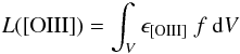 (B.1)where
V is the volume occupied by the outflowing ionized gas,
f the filling factor of the [OIII] emitting clouds in the outflow,
and ϵ [OIII] the [OIII]5007 emissivity that, at the
temperature typical of the NLR (~104 K), has a weak dependence on the
temperature (∝ T0.1). It can be expressed by
(B.1)where
V is the volume occupied by the outflowing ionized gas,
f the filling factor of the [OIII] emitting clouds in the outflow,
and ϵ [OIII] the [OIII]5007 emissivity that, at the
temperature typical of the NLR (~104 K), has a weak dependence on the
temperature (∝ T0.1). It can be expressed by  (B.2)where
hν [OIII] is the energy of the
[OIII]5007 photons (in units of erg), nO + 2 and
ne are the volume densities of the O + 2 ions
and of electrons, respectively (in units of cm-3). Under the reasonable
assumption that most of the oxygen in the ionized outflow is in the O + 2
form, then
(B.2)where
hν [OIII] is the energy of the
[OIII]5007 photons (in units of erg), nO + 2 and
ne are the volume densities of the O + 2 ions
and of electrons, respectively (in units of cm-3). Under the reasonable
assumption that most of the oxygen in the ionized outflow is in the O + 2
form, then  (B.3)where
10 [O/H] gives the oxygen abundance in solar units.
(B.3)where
10 [O/H] gives the oxygen abundance in solar units.
The mass of outflowing ionized gas is given by 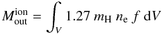 (B.4)\newpage\noindentwhere
mH is the mass of the hydrogen atom, and where we have
neglected the mass contributed by species heavier than helium.
(B.4)\newpage\noindentwhere
mH is the mass of the hydrogen atom, and where we have
neglected the mass contributed by species heavier than helium.
By combining Eqs. (B.1) and (B.4) we obtain 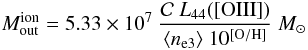 (B.5)where
L44([OIII] ) is the luminosity of the [OIII]5007 line
emitted by the outflow, in units of 1044 erg s-1,
⟨ ne3 ⟩
(= ∫Vne f dV/∫Vf dV)
is the average electron density in the ionized gas clouds, in units of
103 cm-3, and
(B.5)where
L44([OIII] ) is the luminosity of the [OIII]5007 line
emitted by the outflow, in units of 1044 erg s-1,
⟨ ne3 ⟩
(= ∫Vne f dV/∫Vf dV)
is the average electron density in the ionized gas clouds, in units of
103 cm-3, and  is a “condensation factor”,
where
is a “condensation factor”,
where 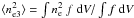 . We
can assume
. We
can assume  under the simplifying hypothesis that all ionizing gas clouds have the same density.
Also, under these assumptions, the mass of outflowing ionized gas is independent of the
filling factor of the emitting clouds.
under the simplifying hypothesis that all ionizing gas clouds have the same density.
Also, under these assumptions, the mass of outflowing ionized gas is independent of the
filling factor of the emitting clouds.
If we assume a simplified model of the outflow (justified by the limited information
currently available to us) where the wind occurs in a conical region, with opening angle
Ω, composed of ionized clouds uniformly distributed and outflowing with velocity
v, out to a radius R, then the mass outflow rate of
ionized gas is given by 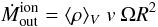 (B.6)where
⟨ ρ ⟩ V is the average mass density in
the whole volume occupied by the outflow, which is given by
(B.6)where
⟨ ρ ⟩ V is the average mass density in
the whole volume occupied by the outflow, which is given by 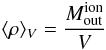 (B.7)where
the volume occupied by the conical outflow is given by
(B.7)where
the volume occupied by the conical outflow is given by
 .
Unless f = 1, generally
⟨ ρ ⟩ V ≠ 1.27 mH ⟨ ne ⟩ ,
since the latter numerical density (defined above) is averaged among the emitting
clouds, not over the whole volume.
.
Unless f = 1, generally
⟨ ρ ⟩ V ≠ 1.27 mH ⟨ ne ⟩ ,
since the latter numerical density (defined above) is averaged among the emitting
clouds, not over the whole volume.
By replacing Eqs. (B.5) and (B.7) into Eq. (B.6) we obtain that the ionized outflow rate is given by
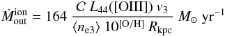 (B.8)where
L44([OIII]), ne3, and
(B.8)where
L44([OIII]), ne3, and
 (≈ 1) were defined above, v3 is the outflow velocity in units of
1000 km s-1, and Rkpc is the radius of the
outflowing region, in units of kpc. The outflow rate is independent of both the opening
angle Ω of the outflow and of the filling factor f of the emitting
clouds (under the assumption of clouds with the same density).
(≈ 1) were defined above, v3 is the outflow velocity in units of
1000 km s-1, and Rkpc is the radius of the
outflowing region, in units of kpc. The outflow rate is independent of both the opening
angle Ω of the outflow and of the filling factor f of the emitting
clouds (under the assumption of clouds with the same density).
The kinetic power (associated with the ionized component) is then given by
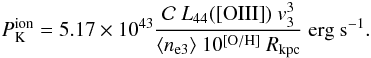 (B.9)
(B.9)
© ESO, 2012
Current usage metrics show cumulative count of Article Views (full-text article views including HTML views, PDF and ePub downloads, according to the available data) and Abstracts Views on Vision4Press platform.
Data correspond to usage on the plateform after 2015. The current usage metrics is available 48-96 hours after online publication and is updated daily on week days.
Initial download of the metrics may take a while.