| Issue |
A&A
Volume 537, January 2012
|
|
|---|---|---|
| Article Number | A41 | |
| Number of page(s) | 10 | |
| Section | The Sun | |
| DOI | https://doi.org/10.1051/0004-6361/201117957 | |
| Published online | 04 January 2012 | |
Online material
Appendix A: Corrections to the eigenfunctions due to the density stratification
In the Appendix we estimate the corrections to the chosen eigenfunctions due to the density stratification. Analytical progress can be made in the small y/χ limit. Since χ is a value smaller than one, this condition would automatically mean that we work in the small y limit, provided χ is not becoming too small. We are interested only in the characteristics of fundamental mode of kink oscillations and its first harmonic. Following Eq. (3) with the boundary conditions vr(L) = dvr(0)/dz = 0 and vr(0) = vr(L) = 0 for the fundamental mode and first harmonic, we introduce a new variable so that
 In the new notations the density inside the loop can be written as
 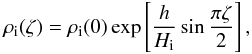 (A.1)where h is the loop height above the solar atmosphere (a similar equation can be written for the external density). Next, we are working in the approximation h/Hi = ϵ ≪ 1, so Eq. (3) becomes
 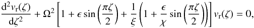 (A.2)where ξ = ρi(0)/ρe(0) > 1 is the density ratio and χ = He/Hi < 1, with He and Hi being the density scale heights inside and outside the loop. Let us we write vr and Ω as
  (A.3)Substituting these expansions into Eq. (A.2) and collecting terms proportional to subsequent powers of ϵ we obtain
 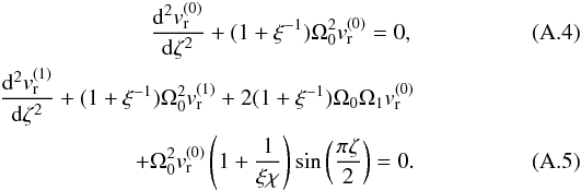 These equations must be solved separately for the fundamental mode and its first harmonic taking into account the boundary conditions.
 (A.6)and
  (A.7)It is important to note that the form of the above solution is exactly the same as the solution we employed for the eigenfunction, vr. In the next order of approximation we obtain Eq. (A.5) which can be written as
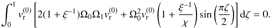
 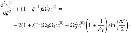 (A.8)This boundary value problem will permit solutions only if the right-hand side satisfies the compatibility condition that can be obtained after multiplying the left-hand side by the expression of
  and integrating with respect to the variable ζ between 0 and 1, or
 After some straightforward calculus we can find that
 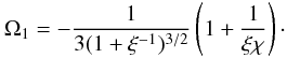 (A.9)As a result, Eq. (A.5) becomes
 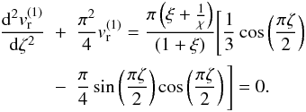 (A.10)This differential equation will have the solution
 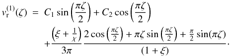 (A.11)Applying the boundary condition
  , we find the constant
 In order to find the value of C2, we use the property of orthogonality, i.e.
 As a result, the first order correction to vr corresponding to the fundamental mode is
  (A.12)In Fig. A.1 we plot the correction to the eigenfunction for ϵ = 0.1, χ = 0.9, and ξ = 10. Figure (A.1) shows that we can approximate vr(z) by cos(πz/2L) since the first order correction brings changes of about 1(%), i.e. insignificant.
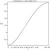 |
Fig. A.1
Correction to the eigenfunction for the fundamental mode kink oscillation when ϵ = 0.1. Here L = 1.5 × 10⁸ m represents the loop length |
| Open with DEXTER | |
A.1. Corrections to the first harmonic
The same analysis can be repeated for the first harmonic, taking into account the right boundary conditions. After a straightforward calculation it is easy to show that  The correction to the eigenfunction corresponding to the first harmonic has been plotted in Fig. A.2 for the same values as before. It is obvious that the changes introduced by stratification in the value of the eigenfunction are of the order of 2(%), i.e. negligably small.
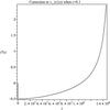 |
Fig. A.2
The same as Fig. A.1 but here we represent the correction to the eigenfunction for the first harmonic kink oscillation. |
| Open with DEXTER | |
The two figures show that the effect of density stratification becomes more important for higher harmonics. Given the very large values of χ we used for prominences, the approximations used in this Appendix will always be valid. Fo the graphical represention of corrections in Figs. A.1 and A.2 we used χ = 1. If we lower this value to, e.g. 0.7 the corrections would still be small since the maximum relative change in the eigenfunction describing the fundamental mode would be 1.1%, while for the first harmonic, this would increase to 3.5%.
The robustness of our analysis was checked using a full numerical investigation for arbitrary values of χ and y. A typical dependence of the P1/P2 period ratio with respect to L/πHi for one value of χ is shown in Fig. A.3 where the solid line corresponds to the analytical and the dotted line represent the numerical results, in both cases the density is inhomogeneous with respect to the coordinate z. The loop is set into motion using a gaussian-shaped source and we use a full reflective boundary conditions at the two footpoints of the loop. After the oscillations are formed, we use the FFT procedure to obtain the values of periods. Our analysis shows that the differences between the results obtained using the variational method and a full numerical investigation are of the order of 7% but towards the large range of L/πHi. Restricting ourself to realistic values, i.e. L/πHi < 5, we see that the results obtained with the two methods coincide with great accuracy.
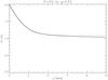 |
Fig. A.3
Comparison of the analytical (solid line) and numerical (dotted line) results for the P1/P2 variation with L/πHi for coronal case corresponding to χ = 0.53. |
| Open with DEXTER | |
© ESO, 2012
Current usage metrics show cumulative count of Article Views (full-text article views including HTML views, PDF and ePub downloads, according to the available data) and Abstracts Views on Vision4Press platform.
Data correspond to usage on the plateform after 2015. The current usage metrics is available 48-96 hours after online publication and is updated daily on week days.
Initial download of the metrics may take a while.