| Issue |
A&A
Volume 537, January 2012
|
|
|---|---|---|
| Article Number | A125 | |
| Number of page(s) | 17 | |
| Section | Planets and planetary systems | |
| DOI | https://doi.org/10.1051/0004-6361/201117701 | |
| Published online | 19 January 2012 | |
Online material
Appendix A: Collision time from friction time
In connection with the presence of gas it is convenient to express the collision time-scale in terms of the gas friction time-scale. In the Epstein drag force regime, valid when the radius of a particle R is smaller than (9/4 times) the mean free path of gas molecules (Weidenschilling 1977), the friction time-scale is  (A.1)Here ρ• is the material density of the particles, while cs and ρg are the sound speed and density of the gas molecules.
The time-scale for a particle of radius Rk to collide with a swarm of particles with physical radius Rj is 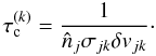 (A.2)where σjk is the mutual collisional cross section. Writing further
  and σjk = π(Rj + Rk)2 and assuming spherical particles we arrive at
 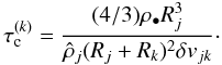 (A.3)In terms of the friction time we get
 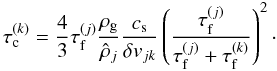 (A.4)For collisions between equal-sized particles, with
  , the expression reduces to
 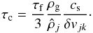 (A.5)A time-dependent numerical solution of a collisional particle system must take collisions into account when choosing the time-step. The time-step criterion of the Monte Carlo collision scheme originates in the requirement that two particles can collide at most once during a time-step, i.e. the collision probability P = δt/τc between any two particles in the same grid cell must be much smaller the unity. This time-step is independent of the maximum density in a grid cell, since particles in dense grid cells have many collision partners and hence can suffer more collisions in the same time-step.
In the streaming instability simulations presented in Sects. 4 and 5 we observe a typical particle rms speed δv ~ 0.025cs. The mass density represented by a single superparticle is  and the friction time is Ωτf = 0.3 (we normalise here by the Keplerian frequency Ω which we define in Sect. 4). This gives Ωτc ≈ 18 from Eq. (A.5). The Courant criterion for the hydrodynamical part of the streaming instability gives the time-step δthydro = 0.000625Ω-1 for 643 and δthydro = 0.0003125Ω-1 for 1283 simulations. Therefore we can ignore the collision time-scale in the simulations when determining the numerical time-step.
A.1. Multiple particle sizes
Equation (A.2) defines the collisional time-scale between particles of two sizes. For two superparticles of equal internal particle number ( ) we have
  , because the cross section σjk and relative speed δvjk are symmetric in (j,k). However, equal particle number per superparticle is numerically expensive, as the mass of a superparticle in that case scales as R3, requiring many more superparticles to represent an equal mass of smaller particles. The second complication is that the collision time-scale becomes very short for smaller particles.
A more common approach is to have equal mass per superparticle. In that case we can define a collision time-scale as the time for all mass in particle j to interact with all mass in particle k. This time-scale is shared between the two particle species and is given by 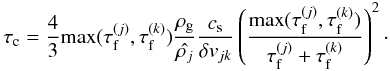 (A.6)To illustrate this, take small particles of friction time
  and large particles of friction time
  . The collision time-scale for the large particles is 100 times shorter than for the small particles, because the superparticle with small physical particles contains 100 times more particles in the swarm. However, the time-scale for collision between a large and a small particle does not imply that all small particles have collided during that time. The correct time-scale is the time for small particles to collide with large particles. When an average small particle has experienced a collision, then all small particles have collided with a large particle, and all the mass in the two superparticles have interacted.
After waiting the common collision time τc, the collision outcome can be solved as if the two colliding particles had equal mass, since effectively a large particle collides with mk/mj small particles during this time. This approach is slightly inconsistent since discrete collisions with N particles of mass mj is not equal to a single collision with a particle of mass Nmj. A collision between a particle of velocity vk and a stationary particle results in the new velocity 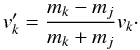 (A.7)After N such collisions the velocity of particle k is
 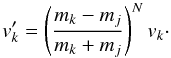 (A.8)In the limit where
 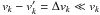 , this equation describes a velocity damping
  (A.9)with characteristic time-scale τd = τc(mk + mj)/(2mj). Completely braking down the large particle requires infinite time, whereas a single discrete collision with an equal-mass particle would remove all the momentum from particle j in one collision time.
To really get the collisional energy equipartition right between particles of different sizes one would have to allow for collisions between a large particle and individual smaller particles. This could either be done by letting superparticles not represent the same mass, but rather the same number of particles. However, this approach would become unpractical to model a large span in particle sizes, since a huge number of superparticles would be required to represent the low-mass particle bins. Alternatively the collision between a swarm of large and small particles could be modelled on the collision time-scale of individual collisions, distributing afterwards the energy and momentum of the particle that suffered the collision among the entire swarm of small particles or among all particle swarms within its mean free path. However, for a large span in particle sizes, this would still require a very small time-step and is therefore unpractical. We simply note here that while collisions between unequal-sized particles can be modelled with the right conservation properties, actual equipartition of particle energies would require an adaptation of the collision algorithm.
Appendix B: Limiting the collision number
During the gravitational contraction of particle clumps the number of particles in a grid cell can become very large, on the order of 1000 s or even 10 000 s. Tracking (1/2)N(N − 1) possible collisions per grid cell then becomes very computationally expensive.
However, particles do not collide with all possible partners during a single time-step. One can limit the number of collision partners, while maintaining the overall collision rate, by sampling only a subset Nmax of the possible collisions. Considering only Nmax out of the N − 1 collision partners for each particle in a grid cell, while increasing the collision probability for each collision partner by (N − 1)/Nmax, yields statistically the same number of collisions.
Consider as an example 101 particles in a grid cell, with the collision probability between any two particles of 10-2. Particle 1 will then on the average collide with 1 other particle. However, calculating the collision probability with 100 other particles is expensive, even when it does not lead to a collision, which is most often the case. Instead we let particle 1 only interact with particles 2 to 6, and give each collision the probability 10-1 instead of 10-2. Particle i has particles i + 1 to i + 5 as collision partners. When reaching particle 97, the collision partners wrap around to particle 1 again, and this way all particles on the average get 10 collision partners (5 of higher index and 5 of lower index) instead of 100.
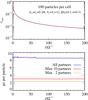 |
Fig. B.1
Evolution of particle rms speed in simulation starting with random motion of amplitude 1. Particles have mean-free-path λ = 0.1 and coefficient of restitution ϵ = 0.3. Drag forces are ignored. The blue line shows the results of a simulation with 100 particles per grid cell and full collision partner list, while the red and golden lines show the results of limiting the collision partners to 10 and 2, respectively, while increasing the collision probability accordingly. The results are extremely similar. The lower panel shows the instantaneous inverse code speed. Limiting the number of collision partners has increased the speed by a factor of approximately three. |
| Open with DEXTER | |
When reducing the number of collision partners, one has to be careful that the particles do not interact only with particles of a nearby index in each time-step. To avoid any such spurious particle preferences, we therefore shuffle the order of particles inside a grid cell in each time-step. We have empirically found that reducing the number of collision partners becomes important when there are more than 100 particles in a grid cell. We show in Fig. B.1 the rms speed of particles undergoing inelastic collisions with coefficient of restitution ϵ = 0.3. We use 100 particles per grid cell and show results where we consider all particles in a cell to be collision partners together with results where we limit the collision partners to 10 and 2. The results are indistinguishable, but the code speed is significantly higher when limiting the number of collision partners (lower panel of Fig. B.1). The typical speed of the Pencil Code for a hydrodynamical simulation with two-way drag forces between gas and particles is ~ 10 μs per particle per time-step. Figure B.1 shows that the computational time needed for superparticle collisions is similar to or lower than the time needed for gas hydrodynamics, particle dynamics, and drag forces, if the number of collision partners is kept below approximately 100.
A side effect of reducing the number of collision partners is that the maximum number of collisions is reduced accordingly. Therefore it be must required that the boosted collision probability P′ = P(N − 1)/Nmax is always much smaller than unity. This must hold for all particle pairs. One can use the maximum relative speed between any two particles within a grid cell to estimate the smallest allowed Nmax that keeps all P′ ≪ 1.
Each swarm in our simulations represents  . The base probability for collision between two superparticle swarms with random motion δv/cs ~ 0.025 is P = δt/τc ~ 10-5 using Eq. (A.5) and a typical hydrodynamical time-step δt at 643 and 1283 resolution. The maximum density reached in the simulations is ρp/ρg ≈ 3000 (see Fig. 7), giving ≈ 13 700 particles in the densest cells. We use Nmax = 100 and thus the maximum boosted probability is P′ ~ 10-3, safely in the regime where the collision time-scale can be ignored when determining the numerical time-step of the code.
Appendix C: From superparticles to inflated particles
Consider a particle component of mass density ρp. A superparticle can maximally hold a particle number  (equivalently particle mass density
  ) that covers the whole area of the grid cell,
  (C.1)Here σ is the cross section of a swarm member and λ is the mean free path of physical particles in the system. This gives a maximum superparticle mass density of
 (C.2)At this mass density the Monte Carlo method breaks down because the superparticle area is larger than a single grid cell (this is not taken into account in the model because collisions are only considered when superparticles share the same grid cell). The free path of a test particle encountering this maximum density superparticle is
 (C.3)using
  . Thus the maximum area criterion coincides with the particle density where the free path is the same as the grid spacing, giving a collision probability of unity when the particle enters a grid cell occupied by a superparticle. This is in fact equivalent to the inflated particle approach, i.e. that overlapping particles always collide.
We still must show that the mean free path of the system is equal to the physical mean free path. The total particle number in the box is  (C.4)
(C.4)
This gives a mean free path for the “grid point particles” of  (C.5)
(C.5)
This shows how the superparticle Monte Carlo method smoothly transforms to the inflated particle method when reducing the number of superparticles and increasing their mass. At the point when the superparticle fills up its grid cell, the collision probability approaches unity inside the cell and the mean free path of the grid cell particles is equal to the mean free path of the physical particles. At the same time one must only allow approaching particles to collide, to avoid multiple collisions inside the grid cell. Of course, the collision detection algorithm for these cubic particles is rather crude, but the geometric effect of considering cubic rather than spherical particles is minor.
© ESO, 2012
Current usage metrics show cumulative count of Article Views (full-text article views including HTML views, PDF and ePub downloads, according to the available data) and Abstracts Views on Vision4Press platform.
Data correspond to usage on the plateform after 2015. The current usage metrics is available 48-96 hours after online publication and is updated daily on week days.
Initial download of the metrics may take a while.