| Issue |
A&A
Volume 536, December 2011
|
|
|---|---|---|
| Article Number | A41 | |
| Number of page(s) | 25 | |
| Section | Interstellar and circumstellar matter | |
| DOI | https://doi.org/10.1051/0004-6361/201117431 | |
| Published online | 05 December 2011 | |
Online material
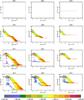 |
Fig. 6
Phase diagrams for the models with Mbh = 107 M⊙ and UV = 0. Temperature is plotted against number density at t = tff = 105 yr. The diagrams are gridded into 752 cells with the weighted masses of the points depicted in color. Red represents a mass of 10 M⊙ or above and blue is for 10-5 M⊙. Isothermal conditions yield a flat profile. From left to right, the cosmic ray rate increases from 1, 100 to 3000 × Galactic. From top to bottom, the X-ray flux increases from 0, 5.1, 28 to 160 erg s-1 cm-2. |
| Open with DEXTER | |
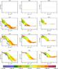 |
Fig. 7
Phase diagrams for the models with Mbh = 106 M⊙ and UV = 0. Temperature is plotted against number density at t = tff = 105 yr. The diagrams are gridded into 752 cells with the weighted masses of the points depicted in color. Red represents a mass of 10 M⊙ or above and blue is for 10-5 M⊙. Isothermal conditions yield a flat profile. From left to right, the cosmic ray rate increases from 1, 100 to 3000 × Galactic. From top to bottom, the X-ray flux increases from 0, 5.1, 28 to 160 erg s-1 cm-2. |
| Open with DEXTER | |
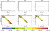 |
Fig. 8
Phase diagrams for the models with Mbh = 108 M⊙ and UV=0. Temperature is plotted against number density at t = tff = 105 yr. The diagrams are gridded into 752 cells with the weighted masses of the points depicted in color. Red represents a mass of 10 M⊙ or above and blue is for 10-5 M⊙. Isothermal conditions yield a flat profile. From left to right, the cosmic ray rate increases from 1, 100 to 3000 × Galactic. From top to bottom, the X-ray flux increases from 0 to 160 erg s-1 cm-2. |
| Open with DEXTER | |
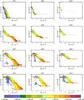 |
Fig. 9
Phase diagrams for the models including UV. The UV flux used in these models is 102.5 G0. Similar to the figures above, Figs. 6 to 8, the images display the temperature against number density at t = tff = 105 yr. The diagrams are gridded into 752 cells with the weighted masses of the points depicted in color. Red represents a mass of 10 M⊙ or above and blue is for 10-5 M⊙. From left to right, the cosmic ray rate increases from 1, 100 to 3000 × Galactic. From top to bottom, the X-ray flux increases from 0 to 160 erg s-1 cm-2. These UV models are simulated for a black hole mass of Mbh = 107 M⊙. |
| Open with DEXTER | |
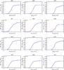 |
Fig. 10
SFEs for the models with Mbh = 107 M⊙ and UV=0. The ratio of the total sink particle mass over the total initial gas mass is plotted against time (in free-fall units). From left to right, the cosmic ray rate increases from 1, 100 to 3000 × Galactic. From top to bottom, the X-ray flux increases from 0, 5.1, 28 to 160 erg s-1 cm-2. The total number of sink particles formed during the run is given in the upper left corner of each panel. |
| Open with DEXTER | |
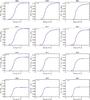 |
Fig. 11
SFEs for the models with Mbh = 106 M⊙ and UV = 0. The ratio of the total sink particle mass over the total initial gas mass is plotted against time (in free-fall units). From left to right, the cosmic ray rate increases from 1, 100 to 3000 × Galactic. From top to bottom, the X-ray flux increases from 0, 5.1, 28 to 160 erg s-1 cm-2. The total number of sink particles formed during the run is given in the upper left corner of each panel. |
| Open with DEXTER | |
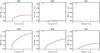 |
Fig. 12
SFEs for the models with Mbh = 108 M⊙ and UV = 0. The ratio of the total sink particle mass over the total initial gas mass is plotted against time (in free-fall units). Note that the y-axis range in this figure differs from the other (SFE) figures. From left to right, the cosmic ray rate increases from 1, 100 to 3000 × Galactic. From top to bottom, the X-ray flux increases from 0 to 160 erg s-1 cm-2. The total number of sink particles formed during the run is given in the upper left corner of each panel. |
| Open with DEXTER | |
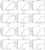 |
Fig. 13
SFEs for the models with UV. The UV flux used in these models is 102.5 G0. Similar to the figures above, Figs. 10 to 12, the images show the ratio of the total sink particle mass over the total initial gas mass and is plotted against time (in free-fall units). From left to right, the cosmic ray rate increases from 1, 100 to 3000 × Galactic. From top to bottom, the X-ray flux increases from 0, 5.1, 28 to 160 erg s-1 cm-2. These UV models are simulated for a a black hole mass of Mbh = 107 M⊙. The total number of sink particles formed during the run is given in the upper left corner of each panel. |
| Open with DEXTER | |
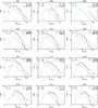 |
Fig. 14
IMFs for the models with Mbh = 107 M⊙ and UV = 0. The images display the time-averaged IMFs between 1 and 3 free-fall times, where tff = 105 yr. From left to right, the cosmic ray rate increases from 1, 100 to 3000 × Galactic. From top to bottom, the X-ray flux increases from 0, 5.1, 28 to 160 erg s-1 cm-2. In each image, for comparison purposes, the Salpeter IMF (green dashed) and the Chabrier IMF (blue dot-dashed) are displayed as fitted to our fiducial model. Two best fits are applied to the data, a linear fit and a lognormal fit, and are shown as purple and red lines. With the exception of the lognormal fit, the slopes above the turn-over mass are given in the upper left corner. |
| Open with DEXTER | |
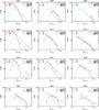 |
Fig. 15
IMFs for the models with Mbh = 106 M⊙ and UV = 0. The images display the time-averaged IMFs between 1 and 3 free-fall times, where tff = 105 yr. From left to right, the cosmic ray rate increases from 1, 100 to 3000 × Galactic. From top to bottom, the X-ray flux increases from 0, 5.1, 28 to 160 erg s-1 cm-2. In each image, for comparison purposes, the Salpeter IMF (green dashed) and the Chabrier IMF (blue dot-dashed) are displayed as fitted to our fiducial model. Two best fits are applied to the data, a linear fit and a lognormal fit, and are shown as purple and red lines. With the exception of the lognormal fit, the slopes above the turn-over mass are given in the upper left corner. |
| Open with DEXTER | |
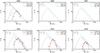 |
Fig. 16
IMFs for the models with Mbh = 108 M⊙ and UV = 0. The images display the time-averaged IMFs between 1 and 3 free-fall times, where tff = 105 yr. From left to right, the cosmic ray rate increases from 1, 100 to 3000 × Galactic. From top to bottom, the X-ray flux increases from 0 to 160 erg s-1 cm-2. In each image, for comparison purposes, the Salpeter IMF (green dashed) and the Chabrier IMF (blue dot-dashed) are displayed as fitted to our fiducial model. Two best fits are applied to the data, a linear fit and a lognormal fit, and are shown as purple and red lines. With the exception of the lognormal fit, the slopes above the turn-over mass are given in the upper left corner. |
| Open with DEXTER | |
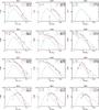 |
Fig. 17
IMFs for the models with UV. The UV flux used in these models is 102.5 G0. Similar to the figures above, Figs. 14 to 16, the images display the time-averaged IMFs between 1 and 3 free-fall times, where tff = 105 yr. From left to right, the cosmic ray rate increases from 1, 100 to 3000 × Galactic. From top to bottom, the X-ray flux increases from 0, 5.1, 28 to 160 erg s-1 cm-2. In each image, for comparison purposes, the Salpeter IMF (green dashed) and the Chabrier IMF (blue dot-dashed) are displayed as fitted to our fiducial model. Two best fits are applied to the data, a linear fit and a lognormal fit, and are shown as purple and red lines. With the exception of the lognormal fit, the slopes above the turn-over mass are given in the upper left corner. These UV models are simulated for a a black hole mass of Mbh = 107 M⊙. |
| Open with DEXTER | |
© ESO, 2011
Current usage metrics show cumulative count of Article Views (full-text article views including HTML views, PDF and ePub downloads, according to the available data) and Abstracts Views on Vision4Press platform.
Data correspond to usage on the plateform after 2015. The current usage metrics is available 48-96 hours after online publication and is updated daily on week days.
Initial download of the metrics may take a while.