| Issue |
A&A
Volume 530, June 2011
|
|
|---|---|---|
| Article Number | L7 | |
| Number of page(s) | 6 | |
| Section | Letters | |
| DOI | https://doi.org/10.1051/0004-6361/201116766 | |
| Published online | 13 May 2011 | |
Online material
Appendix A: Setup of the simulations
A.1. The equilibrium model
As in GD2011, our system represents a zoom around an ionisation region. Since we are computing local simulations, the vertical gravity g = −gez and the kinematic viscosity ν are assumed to be constant. Following our purely radiative model of the κ-mechanism (Gastine & Dintrans 2008a,b), the ionisation region is represented by a temperature-dependent radiative conductivity profile that mimics an opacity bump:

with
 (A.2)where Tbump is the position of the hollow in temperature and σ, e, and
  denote its slope, width, and relative amplitude, respectively. We assume both radiative and hydrostatic equilibria; that is,

where Fbot is the imposed bottom flux. Following GD2011, we chose Lz as the length scale, i.e. [x] = Lz, top density ρtop and top temperature Ttop as density and temperature scales, respectively. The velocity scale is then  , while time is given in units of
  .
.
Table A.1 then summarises the parameters of the numerical simulations presented in this study in these dimensionless units. The penultimate column of this table contains the value of the frequency ω00 of the fundamental unstable radial mode excited by the κ-mechanism, which lies between 3 and 4 for every DNS. The last column gives the value of the Rayleigh number, which quantifies the strength of the convective motions. It is given by

where Lconv is the width of the convective zone, χ = K0/ρ0cp the radiative diffusivity, and s the entropy.
Dimensionless parameters of the numerical simulations.
A.2. The nonlinear equations
With the parallel version of the alternate direction implicit (ADI) solver for the radiative diffusion implemented in the pencil code (see GD2011), we advance the following hydrodynamic equations in time:

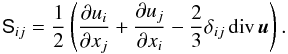
where ρ, u, and T denote density, velocity, and temperature, respectively, while K(T) is given by Eq. (A.1). The operator D/Dt = ∂/∂t + u·∇ is the usual total derivative, while S is the (traceless) rate-of-strain tensor given by
Finally, we impose the condition that all fields are periodic in the horizontal direction, while stress-free boundary conditions (i.e., uz = 0 and dux/dz = 0) are assumed for the velocity in the vertical one. Concerning the temperature, a perfect conductor at the bottom (i.e., flux imposed) and a perfect insulator at the top (i.e., temperature imposed) are applied.
To ensure that both the nonlinear saturation and thermal relaxation are achieved, the simulations were computed over very long times, typically t ≳ 3000. As the eigenfrequency of the unstable acoustic mode ω00 ∈ [3 − 4] (see Table A.1), this corresponds approximately to 1800 periods of oscillation.
© ESO, 2011
Current usage metrics show cumulative count of Article Views (full-text article views including HTML views, PDF and ePub downloads, according to the available data) and Abstracts Views on Vision4Press platform.
Data correspond to usage on the plateform after 2015. The current usage metrics is available 48-96 hours after online publication and is updated daily on week days.
Initial download of the metrics may take a while.