| Issue |
A&A
Volume 521, October 2010
Herschel/HIFI: first science highlights
|
|
|---|---|---|
| Article Number | L24 | |
| Number of page(s) | 7 | |
| Section | Letters | |
| DOI | https://doi.org/10.1051/0004-6361/201015099 | |
| Published online | 01 October 2010 | |
Online Material
AcknowledgementsHIFI has been designed and built by a consortium of institutes and university departments from across Europe, Canada and the United States under the leadership of SRON Netherlands Institute for Space Research, Groningen, The Netherlands and with major contributions from Germany, France and the US. Consortium members are: Canada: CSA, U.Waterloo; France: CESR, LAB, LERMA, IRAM; Germany: KOSMA, MPIfR, MPS; Ireland, NUI Maynooth; Italy: ASI, IFSI-INAF, Osservatorio Astrofisico di Arcetri- INAF; Netherlands: SRON, TUD; Poland: CAMK, CBK; Spain: Observatorio Astronomico Nacional (IGN), Centro de Astrobiologia (CSIC-INTA). Sweden: Chalmers University of Technology - MC2, RSS & GARD; Onsala Space Observatory; Swedish National Space Board, Stockholm University - Stockholm Observatory; Switzerland: ETH Zurich, FHNW; USA: Caltech, JPL, NHSC. The work on star formation at ETH Zurich is partially funded by the Swiss National Science Foundation (grant nr. 200020-113556). This program is made possible thanks to the Swiss HIFI guaranteed time program. This work was supported by the German Deutsche Forschungsgemeinschaft, DFG project number Os 177/1-1. We thank the members of the Herschel key project ``Galactic Cold Cores: A Herschel survey of the source populations revealed by Planck'' lead by M. Juvela (KPOT_mjuvela) for providing us with the results of the SPIRE 250
m mapping and fruitful discussions. We would also like to acknowledge the use of the JCMT CO(3-2) archival data (PI M. Thompson, M08BU15). A portion of this research was performed at the Jet Propulsion Laboratory, California Institute of Technology, under contract with the National Aeronautics and Space administration. We would like to thank an anonymous referee for constructive comments.
Appendix A: Comparison of line profiles taken with different beams
The different lines discussed here were measured at various
telescopes and at different frequencies, so that they all
represent somewhat different spatial resolutions. To allow
a comparison in terms of a physical interpretation, they have
to be translated to a common resolution, so that they stem from
the same area on the sky. As a reference, we use
![]() ,
the
resolution of the KOSMA observations in the 3-2 transition of
the CO isotopes. In principle, all data taken at a finer resolution
can be resampled to this beam if the mapped area is large enough.
,
the
resolution of the KOSMA observations in the 3-2 transition of
the CO isotopes. In principle, all data taken at a finer resolution
can be resampled to this beam if the mapped area is large enough.
Unfortunately, most HIFI observations were only single-point
observations, not full maps, so that such a convolution is
impossible. To derive scaling factors that describe the
translation between the measured intensities and the intensity
that would be obtained in an
![]() beam, we have to assume a
source geometry of the emission. Instead of using any analytic
geometry, we use the actually measured distribution of warm dust
seen in the sub-mm. By assuming that the spatial distribution of
all PDR tracers roughly follows the warm dust, we derive scaling
factors for the line intensities at different beam widths, by
convolving the sub-mm continuum map with the different
beam sizes and picking ratios between the convolved intensities
at the measured positions.
As a continuum map at IRS1, we used the combination of the SPIRE 250
beam, we have to assume a
source geometry of the emission. Instead of using any analytic
geometry, we use the actually measured distribution of warm dust
seen in the sub-mm. By assuming that the spatial distribution of
all PDR tracers roughly follows the warm dust, we derive scaling
factors for the line intensities at different beam widths, by
convolving the sub-mm continuum map with the different
beam sizes and picking ratios between the convolved intensities
at the measured positions.
As a continuum map at IRS1, we used the combination of the SPIRE 250 ![]() m
(
m
(
![]() beam size
beam size![]() ) and SCUBA 450
) and SCUBA 450 ![]() m image (
m image (
![]() beam size, Holland et al. 1999), because IRS1 is saturated in SPIRE
250
beam size, Holland et al. 1999), because IRS1 is saturated in SPIRE
250 ![]() m, whereas the observed area of SCUBA 450
m, whereas the observed area of SCUBA 450 ![]() m is too small
to make a convolution map with the beam size of
m is too small
to make a convolution map with the beam size of
![]() .
We regrid
the SCUBA 450
.
We regrid
the SCUBA 450 ![]() m image to the same grid as SPIRE 250
m image to the same grid as SPIRE 250 ![]() m, determine
the scaling factor between the SCUBA 450
m, determine
the scaling factor between the SCUBA 450 ![]() m and the SPIRE 250
m and the SPIRE 250 ![]() m
maps from the overlapping area, and replace the saturated pixels
of SPIRE 250
m
maps from the overlapping area, and replace the saturated pixels
of SPIRE 250 ![]() m with the scaled SCUBA data.
As this combination implies some arbitrariness, we tested
four different approaches. We derive the scaling factor
in a least squares fit using either (1) all the valid overlapping pixels
or (2) only overlapping pixels with SPIRE 250
m with the scaled SCUBA data.
As this combination implies some arbitrariness, we tested
four different approaches. We derive the scaling factor
in a least squares fit using either (1) all the valid overlapping pixels
or (2) only overlapping pixels with SPIRE 250 ![]() m
>100 Jy/beam. When replacing
SPIRE pixels, we replace either (1) only saturated pixels,
or (2) the full square area (
m
>100 Jy/beam. When replacing
SPIRE pixels, we replace either (1) only saturated pixels,
or (2) the full square area (
![]() pixels)
containing
all saturated pixels. The combination of these provide 4 different
beam scaling factors, which are consistent to within 3%. Taking
the average of these 4 values, we derive the final factors
as shown in Table A.1.
A direct convolution to
pixels)
containing
all saturated pixels. The combination of these provide 4 different
beam scaling factors, which are consistent to within 3%. Taking
the average of these 4 values, we derive the final factors
as shown in Table A.1.
A direct convolution to
![]() was possible for the ground-based
maps that were observed with a smaller beam, such as the JCMT
CO(3-2) map. All the resulting intensities are summarized in Table A.2.
was possible for the ground-based
maps that were observed with a smaller beam, such as the JCMT
CO(3-2) map. All the resulting intensities are summarized in Table A.2.
Table A.1:
The scaling factors between the different beam size observations, which
should be multiplied to the line intensity to estimate the one in a
![]() beam.
beam.
![\begin{figure}
\par\hspace*{2mm}\includegraphics[angle=0.0,width=9cm]{15099fig4.eps}
\end{figure}](/articles/aa/olm/2010/13/aa15099-10/img54.png)
|
Figure A.1:
a) The spatial distribution of warm dust obtained by combining
the SPIRE 250 |
| Open with DEXTER | |
Table A.2: List of the complementary data.
Appendix B: The clumpy PDR model
To model the far-infrared line emission from S140, we used a superposition
of spherical clumps described by the KOSMA-![]() PDR model (Röllig et al. 2006)
that represent an ensemble of clumps with a fixed size-spectrum (Cubick et al. 2008).
The KOSMA-
PDR model (Röllig et al. 2006)
that represent an ensemble of clumps with a fixed size-spectrum (Cubick et al. 2008).
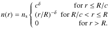
The KOSMA-![]() PDR model simulates a spherical cloud with a radial
density profile given by
PDR model simulates a spherical cloud with a radial
density profile given by
|
(B.1) |
The constant c determines the dynamic range that is covered by the power-law density decay. The spectrum of PDR clumps is characterized by the clump mass spectrum

|
(B.2) |
where the factor a is determined by the total mass of clumps within the beam,
| (B.3) |
which implicitly defines the surface density of the individual clumps
Every individual clump is treated as a spherically symmetric configuration
illuminated by an isotropic external UV radiation field, specified in terms
of the average interstellar radiation field,
![]() erg cm-2 s-1 in Draine units, and cosmic rays
producing an average ionization rate,
erg cm-2 s-1 in Draine units, and cosmic rays
producing an average ionization rate,
![]() s-1. The internal velocity
dispersion of molecules within the clumps is fixed to 1 km s-1.
The model computes the stationary chemical and temperature
structure by solving the coupled detailed balance of heating,
line and continuum cooling, and the chemical network using the
UMIST data base of reaction rates (Woodall et al. 2007) expanded by separate
entries for the 13C chemistry (see Röllig et al. 2007, for details).
The chemical network currently does not include 18O, so that
C18O predictions can only be obtained by scaling the 13CO
values ignoring fractionation between the two species. As this ignores the different
self-shielding of 13CO and C18O, the model results for C18O
are less reliable than for the other lines.
s-1. The internal velocity
dispersion of molecules within the clumps is fixed to 1 km s-1.
The model computes the stationary chemical and temperature
structure by solving the coupled detailed balance of heating,
line and continuum cooling, and the chemical network using the
UMIST data base of reaction rates (Woodall et al. 2007) expanded by separate
entries for the 13C chemistry (see Röllig et al. 2007, for details).
The chemical network currently does not include 18O, so that
C18O predictions can only be obtained by scaling the 13CO
values ignoring fractionation between the two species. As this ignores the different
self-shielding of 13CO and C18O, the model results for C18O
are less reliable than for the other lines.
In the superposition of clumps, the line emission from the different
clumps is simply added assuming that the velocity dispersion between
the clumps is large enough, so that they do not shield each other in
position-velocity space. This is valid for most species, except for the [O I]
emission, which is opticallyvery thick (
![]() ), so that
the lines are much broader than the velocity distribution. Therefore,
the model is unable to provide any reliable estimate of the
[O I] intensities. For the continuum extinction of the UV
radiation, the situation is different. There, mutual shading of the
clouds is relevant, leading to the concept of different clump
ensembles that ``see'' different UV fields if the average ensemble
extinction exceeds an
), so that
the lines are much broader than the velocity distribution. Therefore,
the model is unable to provide any reliable estimate of the
[O I] intensities. For the continuum extinction of the UV
radiation, the situation is different. There, mutual shading of the
clouds is relevant, leading to the concept of different clump
ensembles that ``see'' different UV fields if the average ensemble
extinction exceeds an ![]() of about unity.
of about unity.
The parameters of the clump mass spectrum imply that most of the
mass is actually contained in the largest clumps that also have
the maximum column density or ![]() ,
respectively. The dependence of
,
respectively. The dependence of ![]() and clump size on clump mass is given by
and clump size on clump mass is given by
![\begin{displaymath}R = 5.3 \times 10^{18} \left( \frac{M [M_{\odot}] }{n [{\rm cm}^{-3}]} \right)^{\frac{1}{3}}
\end{displaymath}](/articles/aa/olm/2010/13/aa15099-10/img68.png)
|
(B.4) |
and
![\begin{displaymath}A_{\rm V} =1.6018 \times 10^{21} n[{\rm cm}^{-3}] R\rm [cm].
\end{displaymath}](/articles/aa/olm/2010/13/aa15099-10/img69.png)
|
(B.5) |
In terms of the total clump surface or the total solid angle of the different clumps, we find about equal contributions from each logarithmic mass bin in the ensemble (Eq. (16) in Cubick et al. 2008). Consequently, we find a non-trivial dependence of the intensity in the different HIFI lines on the clump mass. Figures 3 and 5 from Cubick et al. (2008) show that the [C II] emission is dominated by the largest clumps, while the high-J CO lines are dominated by the smallest clumps. A complex, non-monotonic behavior is observed for the lines from atomic oxygen and mid- to low-J CO isotopes.
As the clump spectrum is purely observationally based, it has no direct relation to a stability criterion. We indeed find that both the most massive clumps are unstable to gravitational collapse and that the smallest clumps will be dispersed on the timescale of a few million years. Therefore, the spectrum can only be considered as a snapshot of interstellar turbulence that reflects the density structure over a timescale of 106-107 years. The assumption of a steady-state chemistry and energy-balance is therefore only applicable if all rates are higher. This holds for the dense clumps in the S140 model fit with densities above 104 cm-3, but for lower densities, an explicitly time-dependent modeling would be required (Viti et al. 2006).
Current usage metrics show cumulative count of Article Views (full-text article views including HTML views, PDF and ePub downloads, according to the available data) and Abstracts Views on Vision4Press platform.
Data correspond to usage on the plateform after 2015. The current usage metrics is available 48-96 hours after online publication and is updated daily on week days.
Initial download of the metrics may take a while.